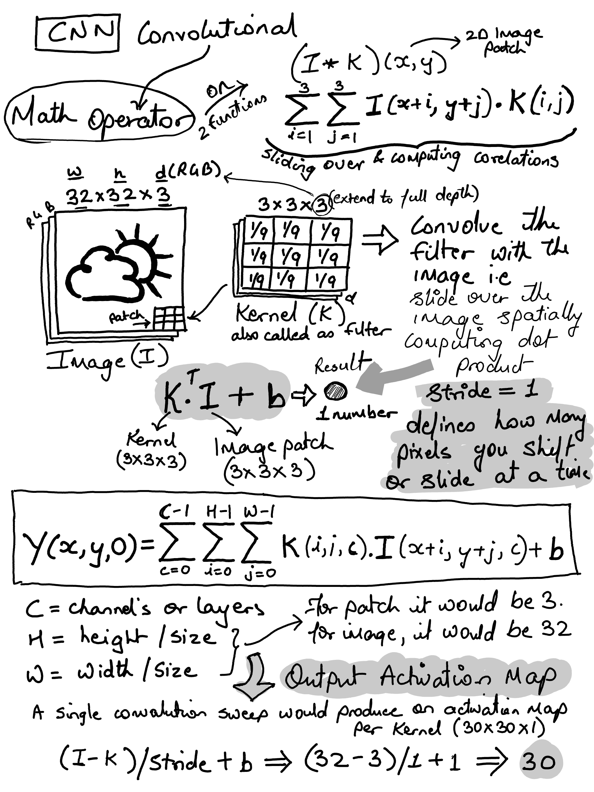
◉ CNN (Convolutional Neural Networks)#
CIFAR-10 dataset#
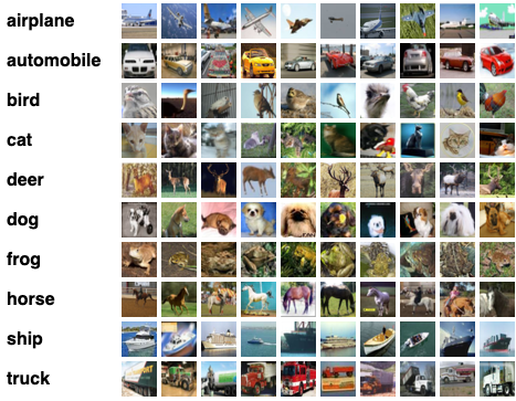
CIFAR-10 dataset consists of 60000 32x32 colour images in 10 classes, with 6000 images per class. There are 50000 training images and 10000 test images.
import os
import tarfile
import pickle
from pathlib import Path

import numpy as np
import matplotlib.pyplot as plt
class_names = ['airplane', 'automobile', 'bird', 'cat', 'deer',
               'dog', 'frog', 'horse', 'ship', 'truck']
import urllib.request

DATA_DIR = Path("./data")
DATA_DIR.mkdir(parents=True, exist_ok=True)

url = "https://www.cs.toronto.edu/~kriz/cifar-10-python.tar.gz"
tgz_path = DATA_DIR / "cifar-10-python.tar.gz"
extract_dir = DATA_DIR

if not tgz_path.exists():
    print("Downloading...")
    urllib.request.urlretrieve(url, tgz_path)

print("Extracting...")
with tarfile.open(tgz_path, "r:gz") as tar:
    tar.extractall(path=extract_dir)

cifar_dir = extract_dir / "cifar-10-batches-py"
print("CIFAR dir:", cifar_dir, "exists?", cifar_dir.exists())
Extracting...
/var/folders/hr/kvb_nv256v958_chgsmxrsdm0000gn/T/ipykernel_65363/2772982909.py:16: DeprecationWarning: Python 3.14 will, by default, filter extracted tar archives and reject files or modify their metadata. Use the filter argument to control this behavior.
  tar.extractall(path=extract_dir)
CIFAR dir: data/cifar-10-batches-py exists? True
CIFAR batches were pickled in python2, so Python3 needs encoding=”bytes” or “latin1”#
def unpickle(path: Path) -> dict:
    with open(path, "rb") as f:
        return pickle.load(f, encoding="bytes")

sorted([p.name for p in cifar_dir.iterdir()])
['batches.meta',
 'data_batch_1',
 'data_batch_2',
 'data_batch_3',
 'data_batch_4',
 'data_batch_5',
 'readme.html',
 'test_batch']
data_batch_1 = unpickle(cifar_dir / "data_batch_1")
print(data_batch_1.keys())
print("Batch 1 shape: ",data_batch_1[b"data"].shape)
print("First 10 labels: ",[class_names[label] for label in data_batch_1[b"labels"][:10]])
dict_keys([b'batch_label', b'labels', b'data', b'filenames'])
Batch 1 shape:  (10000, 3072)
First 10 labels:  ['frog', 'truck', 'truck', 'deer', 'automobile', 'automobile', 'bird', 'horse', 'ship', 'cat']
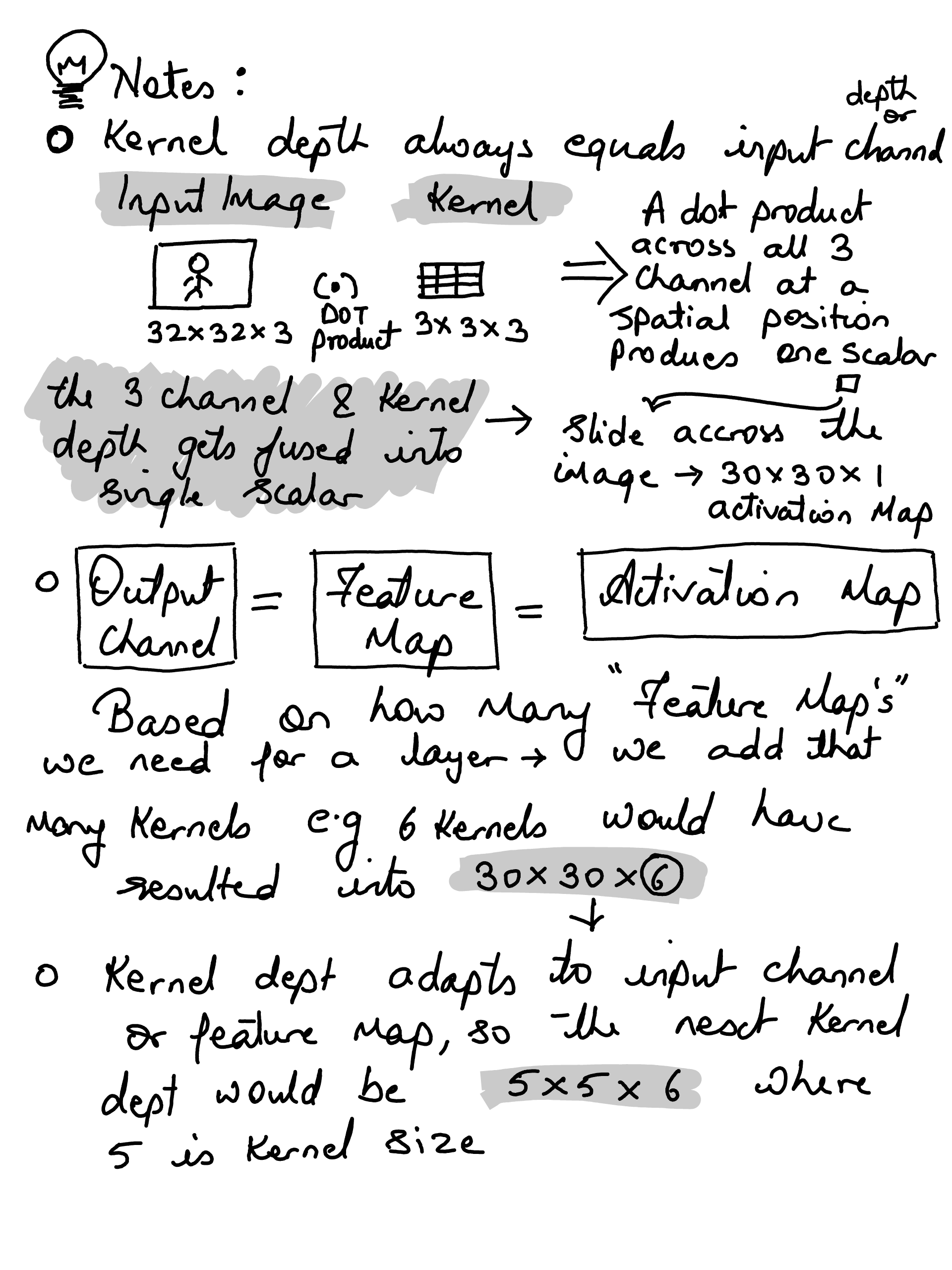
CIFAR stores R, G and B flat - each 1024 bytes i.e. R = 32x32 = 1024. Combining all 3 channels would be 3072 bytes. Our next task is to convert “flat 3072” bytes into real images (N, 32, 32, 3) where N is the number of samples#
def to_image(x_flat: np.ndarray) -> np.ndarray:
    x = x_flat.reshape(-1, 3, 32, 32)          # (N, C, H, W)
    x = np.transpose(x, (0, 2, 3, 1))          # (N, H, W, C)
    return x

x_batch1 = to_image(data_batch_1[b"data"])
y_batch1 = np.array(data_batch_1[b"labels"])

x_batch1.shape, x_batch1.dtype,y_batch1.shape, y_batch1.dtype
((10000, 32, 32, 3), dtype('uint8'), (10000,), dtype('int64'))
Visualize one sample image on a 32x32 grid#
# index = np.random.randint(0, 10000)
sample = 4667
plt.imshow(x_batch1[sample])
plt.title(f"label: {class_names[y_batch1[sample]]}, idx: {y_batch1[sample]}")
# plt.axis('off')
plt.show()

Lets load all the 5 training batches and 1 test batch from CIFAR#
# Loading testing batch
test_batch = unpickle(cifar_dir / "test_batch")
X_test = to_image(test_batch[b"data"])
y_test = np.array(test_batch[b"labels"])

X_test.shape, y_test.shape
((10000, 32, 32, 3), (10000,))
# Training batch...
xs, ys = [], []
for i in range(1, 6):
    batch = unpickle(cifar_dir / f"data_batch_{i}")
    x = to_image(batch[b"data"])
    y = np.array(batch[b"labels"])
    xs.append(x)
    ys.append(y)

X_train = np.concatenate(xs, axis=0)
y_train = np.concatenate(ys, axis=0)

X_train.shape, y_train.shape
((50000, 32, 32, 3), (50000,))
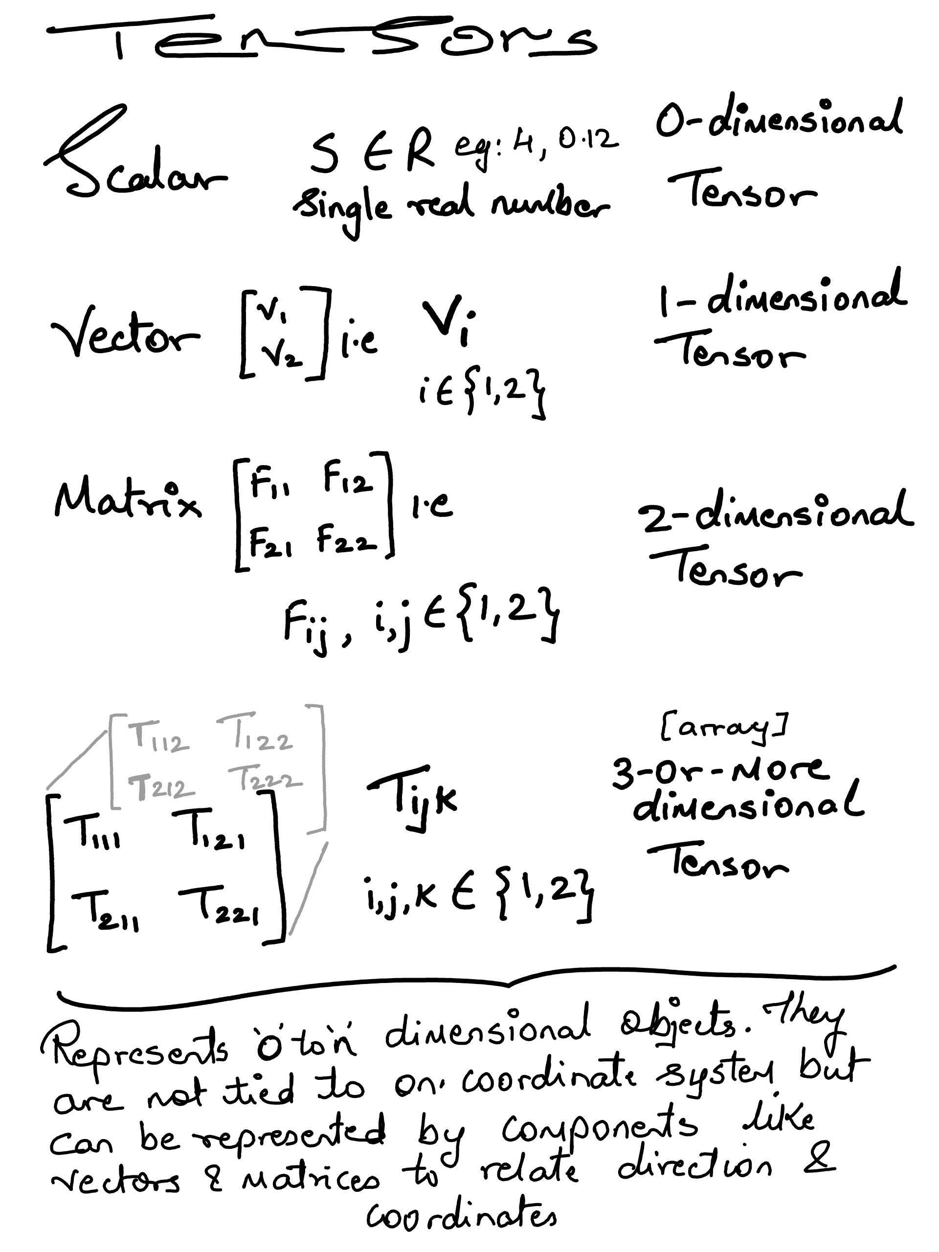
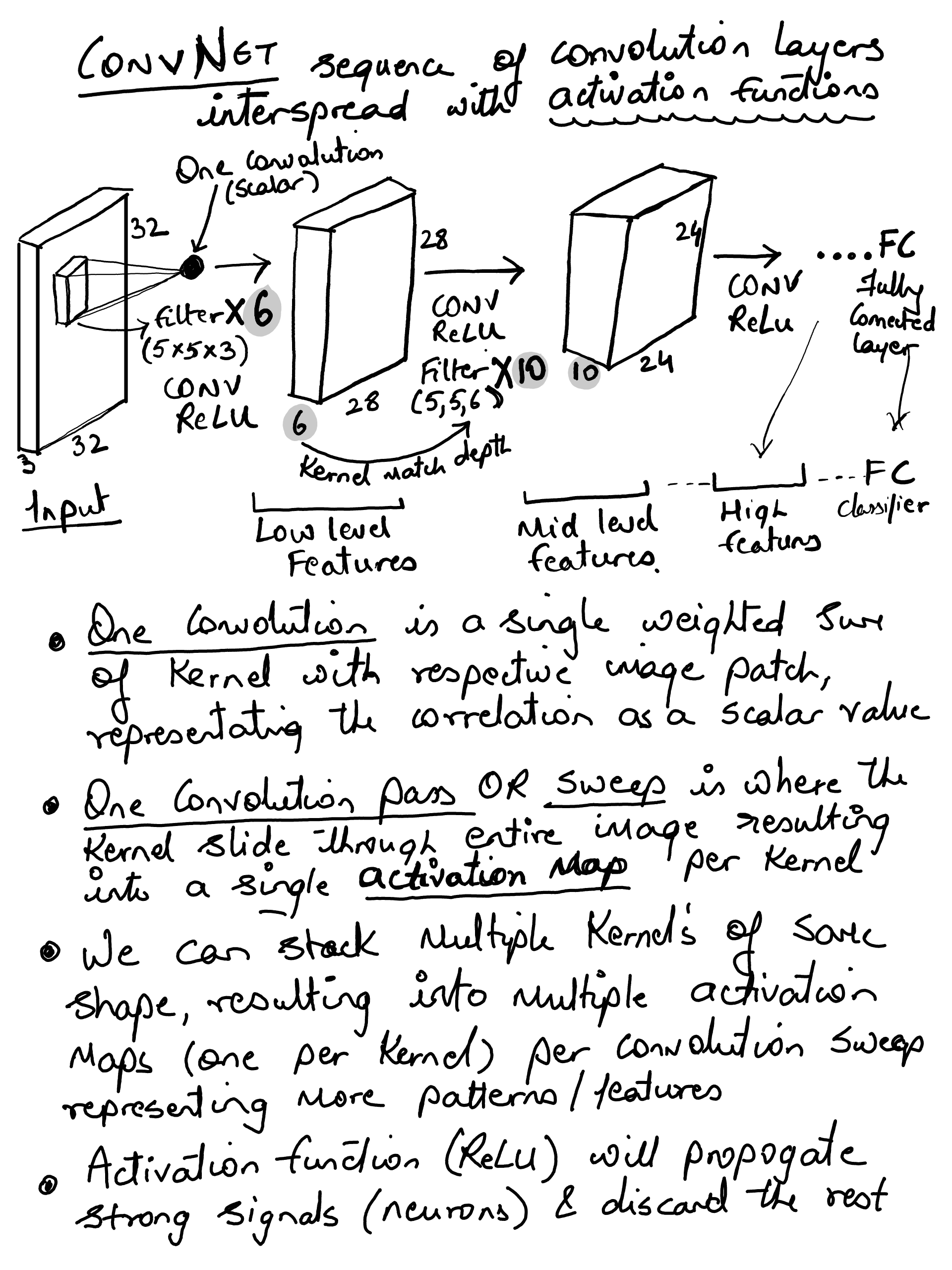
ConvNet#
The goal to build a simple ConvNet using PyTorch and train it on CIFAR 10 dataset. I wanted to visualize all the layers to look at the activation map. Lets consider below pipeline
input(32×32×3) → conv/relu → pool → conv/relu → pool → conv/relu → pool → FC
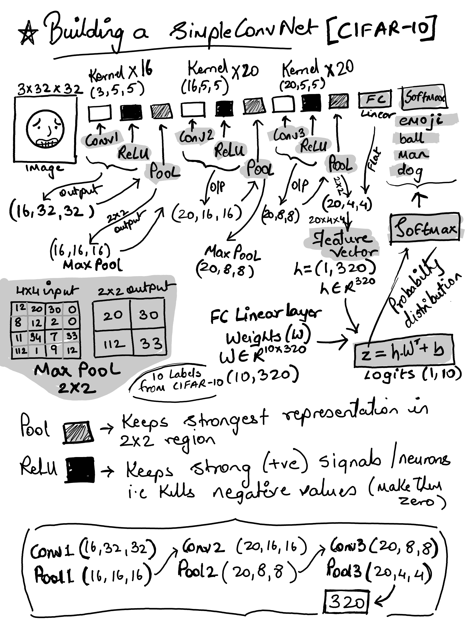
max pooling with 2x2 window and a stride of 2 would reduce each 4 pixels to 1 i.e. `max (a, b, c, d). So it keeps the largest activations and discard the rest reducing the overall spatial features by 75% (in other words, reducing the height and width by 50% each)
note: writing depth/channel/batch first is pytorch style of tensor representation
import torch
import torch.nn as nn
import torch.nn.functional as F

device = "cuda" if torch.cuda.is_available() else "cpu"
device
'cpu'
import torch.nn as nn
import torch.nn.functional as F

class SimpleConvNet(nn.Module):
    def __init__(self, num_classes=10):
        super().__init__()
        self.conv1 = nn.Conv2d(3, 16, kernel_size=5, stride=1, padding=2)
        self.relu1 = nn.ReLU(inplace=False)
        self.pool1 = nn.MaxPool2d(kernel_size=2, stride=2)

        self.conv2 = nn.Conv2d(16, 20, kernel_size=5, stride=1, padding=2)
        self.relu2 = nn.ReLU(inplace=False)
        self.pool2 = nn.MaxPool2d(kernel_size=2, stride=2)

        self.conv3 = nn.Conv2d(20, 20, kernel_size=5, stride=1, padding=2)
        self.relu3 = nn.ReLU(inplace=False)
        self.pool3 = nn.MaxPool2d(kernel_size=2, stride=2)

        self.fc = nn.Linear(20 * 4 * 4, num_classes)

    def forward(self, x):
        x = self.conv1(x)
        x = self.relu1(x)
        x = self.pool1(x)

        x = self.conv2(x)
        x = self.relu2(x)
        x = self.pool2(x)

        x = self.conv3(x)
        x = self.relu3(x)
        x = self.pool3(x)

        x = torch.flatten(x, 1)
        x = self.fc(x)
        return x

model = SimpleConvNet().to(device)

print("conv(n) = (input depth, no of kernels, kernel size, stride, padding))\n")
print(model)
conv(n) = (input depth, no of kernels, kernel size, stride, padding))

SimpleConvNet(
  (conv1): Conv2d(3, 16, kernel_size=(5, 5), stride=(1, 1), padding=(2, 2))
  (relu1): ReLU()
  (pool1): MaxPool2d(kernel_size=2, stride=2, padding=0, dilation=1, ceil_mode=False)
  (conv2): Conv2d(16, 20, kernel_size=(5, 5), stride=(1, 1), padding=(2, 2))
  (relu2): ReLU()
  (pool2): MaxPool2d(kernel_size=2, stride=2, padding=0, dilation=1, ceil_mode=False)
  (conv3): Conv2d(20, 20, kernel_size=(5, 5), stride=(1, 1), padding=(2, 2))
  (relu3): ReLU()
  (pool3): MaxPool2d(kernel_size=2, stride=2, padding=0, dilation=1, ceil_mode=False)
  (fc): Linear(in_features=320, out_features=10, bias=True)
)
With input being (3,32,32) - the output shape of each layers
(16,32,32) conv1/relu
(16,16,16) pool1
(20,16,16) conv2/relu
(20,8,8) pool2
(20,8,8) conv3/relu
(20,4,4) pool3
(320,) FC (feature vector)
(10,) logits
(10,) softmax probability distribution
Model Parameters (weights and bias)#
total_params = sum(p.numel() for p in model.parameters() if p.requires_grad)
print(f"==> Total Trainable Params: {total_params:,}\n")

print("--- Parameters per layer ---")
for name, module in model.named_modules():
    if isinstance(module, (nn.Conv2d, nn.Linear)):
        print(f"[{name}]", "-" * 70)

        # 1. Print Hyperparameters
        if isinstance(module, nn.Conv2d):
            print(f"  Config:  Kernel {module.kernel_size}   |   Stride {module.stride}   |   Padding {module.padding}")
        elif isinstance(module, nn.Linear):
            print(f"  Config:  In {module.in_features} -> Out {module.out_features}")

        for p_name, p_tensor in module.named_parameters(recurse=False):
            print(f"  Param:   {p_name:<10}   |   Shape: {str(p_tensor.shape):<20}   |   Count: {p_tensor.numel()}")
==> Total Trainable Params: 22,466

--- Parameters per layer ---
[conv1] ----------------------------------------------------------------------
  Config:  Kernel (5, 5)   |   Stride (1, 1)   |   Padding (2, 2)
  Param:   weight       |   Shape: torch.Size([16, 3, 5, 5])   |   Count: 1200
  Param:   bias         |   Shape: torch.Size([16])       |   Count: 16
[conv2] ----------------------------------------------------------------------
  Config:  Kernel (5, 5)   |   Stride (1, 1)   |   Padding (2, 2)
  Param:   weight       |   Shape: torch.Size([20, 16, 5, 5])   |   Count: 8000
  Param:   bias         |   Shape: torch.Size([20])       |   Count: 20
[conv3] ----------------------------------------------------------------------
  Config:  Kernel (5, 5)   |   Stride (1, 1)   |   Padding (2, 2)
  Param:   weight       |   Shape: torch.Size([20, 20, 5, 5])   |   Count: 10000
  Param:   bias         |   Shape: torch.Size([20])       |   Count: 20
[fc] ----------------------------------------------------------------------
  Config:  In 320 -> Out 10
  Param:   weight       |   Shape: torch.Size([10, 320])   |   Count: 3200
  Param:   bias         |   Shape: torch.Size([10])       |   Count: 10
Prepare test and training data#
Our current Input shape is X.shape == (num_images, height, width, channels) e.g. (N, 32, 32, 3) but PyTorch ConvNets expects a different shape i.e. (N, channels, height, width) e.g (N, 3, 32, 32)
premute(0,3,1,2) would reorders (N, H, W, C) → (N, C, H, W)
(note
/ 255.0normalizes pixel values)
from torch.utils.data import TensorDataset
from torch.utils.data import DataLoader

batch_size = 128

Xtr = torch.from_numpy(X_train).permute(0,3,1,2).float() / 255.0
ytr = torch.from_numpy(y_train).long()
Xte = torch.from_numpy(X_test).permute(0,3,1,2).float() / 255.0
yte = torch.from_numpy(y_test).long()

train_loader = DataLoader(TensorDataset(Xtr, ytr), batch_size=batch_size, shuffle=True)
test_loader  = DataLoader(TensorDataset(Xte, yte), batch_size=batch_size, shuffle=False)

print("Batch size:", batch_size)
print("Train batches:", len(train_loader), "Test batches:", len(test_loader))
Batch size: 128
Train batches: 391 Test batches: 79
Train and Evaluate#
Each epoch would still go over entire dataset (50K CIFAR samples) - so with batch_size 128, we will have 390 batches. The train_loader would scoop in 128 in each iteration…
current_epoch = 0
total_epochs = 15

import time

optimizer = torch.optim.SGD(model.parameters(), lr=0.01, momentum=0.9, weight_decay=5e-4)

loss_fn = nn.CrossEntropyLoss()

def calculate_loss_accuracy(running_loss, correct, total):
    epoch_loss = running_loss / total
    epoch_acc = correct / total
    return epoch_loss, epoch_acc

def train(epoch):
    model.train()
    running_loss = 0.0
    correct = 0
    total = 0
    start_time = time.time()

    # one mini batch at a time...
    for batch_idx, (x, y) in enumerate(train_loader):

        # move to device
        x, y = x.to(device), y.to(device)
        optimizer.zero_grad()  # reset gradients

        logits = model(x) # forward pass
        loss = loss_fn(logits, y) # compute loss

        loss.backward() # backpropagation
        optimizer.step() # update parameters, we are using Stochastic Gradient Descent -> weight = weight - lr * grad (plus momentum/weight_decay)

        running_loss += loss.item() * x.size(0)
        total += x.size(0)

        correct += (logits.argmax(dim=1) == y).sum().item()

    epoch_loss, epoch_acc = calculate_loss_accuracy(running_loss, correct, total)
    elapsed = time.time() - start_time
    return epoch_loss, epoch_acc, elapsed

def evaluate(loader):
    model.eval()
    running_loss = 0.0
    correct = 0
    total = 0

    with torch.no_grad():
        for x, y in loader:
            x, y = x.to(device), y.to(device)
            logits = model(x)
            loss = loss_fn(logits, y)

            running_loss += loss.item() * x.size(0)
            total += x.size(0)

            correct += (logits.argmax(dim=1) == y).sum().item()

    test_loss, test_accuracy = calculate_loss_accuracy(running_loss, correct, total)
    return test_loss, test_accuracy

def run_one_epoch():
    global current_epoch
    current_epoch = current_epoch + 1

    epoch_loss, epoch_acc, elapsed = train(current_epoch)
    test_loss, test_acc = evaluate(test_loader)

    print(f"Train Epoch {current_epoch}/{total_epochs} - Time: {elapsed:.2f}s \n==>"
        f"Training Loss: {epoch_loss:.4f} - "
        f"Training Accuracy: {epoch_acc*100:.2f}% - "
        f"Test Loss: {test_loss:.4f} - "
        f"Test Accuracy: {test_acc*100:.2f}%")
Single Epoch Run#
run_one_epoch()
Train Epoch 1/15 - Time: 20.27s
==>Training Loss: 2.0125 - Training Accuracy: 25.67% - Test Loss: 1.7398 - Test Accuracy: 36.02%
Lets do some inference - the model will perform bogus… I promise#
some visualization functions to show activations of output labels with progress bar…
import matplotlib.pyplot as plt

def denorm_cifar(img_chw):
    mean = torch.tensor([0.4914, 0.4822, 0.4465]).view(3,1,1)
    std  = torch.tensor([0.2470, 0.2435, 0.2616]).view(3,1,1)
    return img_chw * std + mean

# we normalized during dataset creation, we need to de-normalize for display
def denorm_if_needed(img_chw):
    mean = torch.tensor([0.4914, 0.4822, 0.4465]).view(3,1,1)
    std  = torch.tensor([0.2470, 0.2435, 0.2616]).view(3,1,1)
    return (img_chw * std + mean).clamp(0, 1)

def show_predictions(
    x_batch, y_true, probs,
    n=12, cols=2, topk=5,
    font=16, fig_scale=1.0
):
    x_cpu = x_batch.detach().cpu()
    y_cpu = y_true.detach().cpu()
    p_cpu = probs.detach().cpu()

    pred = p_cpu.argmax(dim=1)
    rows = (n + cols - 1) // cols
    total_cols = cols * 2

    fig = plt.figure(figsize=(total_cols * 5.5 * fig_scale, rows * 4.2 * fig_scale))
    gs = fig.add_gridspec(rows, total_cols, width_ratios=[1.25, 1.0] * cols, wspace=0.25, hspace=0.5)

    for i in range(n):
        r = i // cols
        c = i % cols

        ax_img = fig.add_subplot(gs[r, c*2])
        ax_bar = fig.add_subplot(gs[r, c*2 + 1])

        # ----- image -----
        img_t = x_cpu[i]
        # If values look normalized (roughly centered around 0), de-normalize; else show as-is.
        if img_t.min() < 0 or img_t.max() > 1:
            img_t = denorm_cifar(img_t)   # only if you actually normalized earlier

        img = img_t.clamp(0, 1).permute(1,2,0).numpy()

        ax_img.imshow(img)
        ax_img.axis("off")

        gt_idx = int(y_cpu[i])
        pr_idx = int(pred[i])
        ok = (gt_idx == pr_idx)

        gt = class_names[gt_idx]
        pr = class_names[pr_idx]

        ax_img.set_title(
            f"ground truth: {gt}  |  pred: {pr}",
            fontsize=font, pad=10
        )

        # ----- top-k bars -----
        vals, idxs = torch.topk(p_cpu[i], k=topk)

        # reverse so the biggest ends up at the TOP after invert_yaxis()
        vals = vals.numpy()[::-1]
        idxs = idxs.numpy()[::-1]
        labels = [class_names[j] for j in idxs]

        # Colors: if correct => GT bar green (if present), others red. if incorrect => all red.
        colors = []
        for cls_idx in idxs:
            if ok and int(cls_idx) == gt_idx:
                colors.append("green")
            else:
                colors.append("red")

        y_pos = np.arange(topk)
        bars = ax_bar.barh(y_pos, vals, color=colors)

        ax_bar.set_yticks(y_pos)
        ax_bar.set_yticklabels(labels, fontsize=font-2)
        ax_bar.set_xlim(0, 1.0)
        ax_bar.tick_params(axis="x", labelsize=font-2)
        ax_bar.set_xlabel("prob", fontsize=font-2)

        # values at end of bars
        for b, v in zip(bars, vals):
            ax_bar.text(
                min(v + 0.02, 0.98),
                b.get_y() + b.get_height()/2,
                f"{v:.2f}",
                va="center",
                fontsize=font-2
            )

        ax_bar.invert_yaxis()

    plt.tight_layout()
    plt.show()
cherry pick 200 samples from test data and calcualte accuracy… The seed will ensure same sample for each epoch so that we can see it building up to confidence…
import torch
import numpy as np

def test_random_200():
    np.random.seed(24)
    idx200 = np.random.choice(len(Xte), size=200, replace=False)

    x200 = Xte[idx200].to(device)   # (200,3,32,32)
    y200 = yte[idx200].to(device)   # (200,)

    # set model to eval mode and get predictions
    model.eval()
    with torch.no_grad():
        logits200 = model(x200)
        probs200 = torch.softmax(logits200, dim=1)

    # calculate accuracy on these 200
    acc200 = (probs200.argmax(dim=1) == y200).float().mean().item()
    print("\n==> Test accuracy on random 200 from test set:", round(acc200, 4))

    show_predictions(
        x200, y200, probs200,
        n=20, cols=2, topk=5,
        font=14, fig_scale=1.0
    )
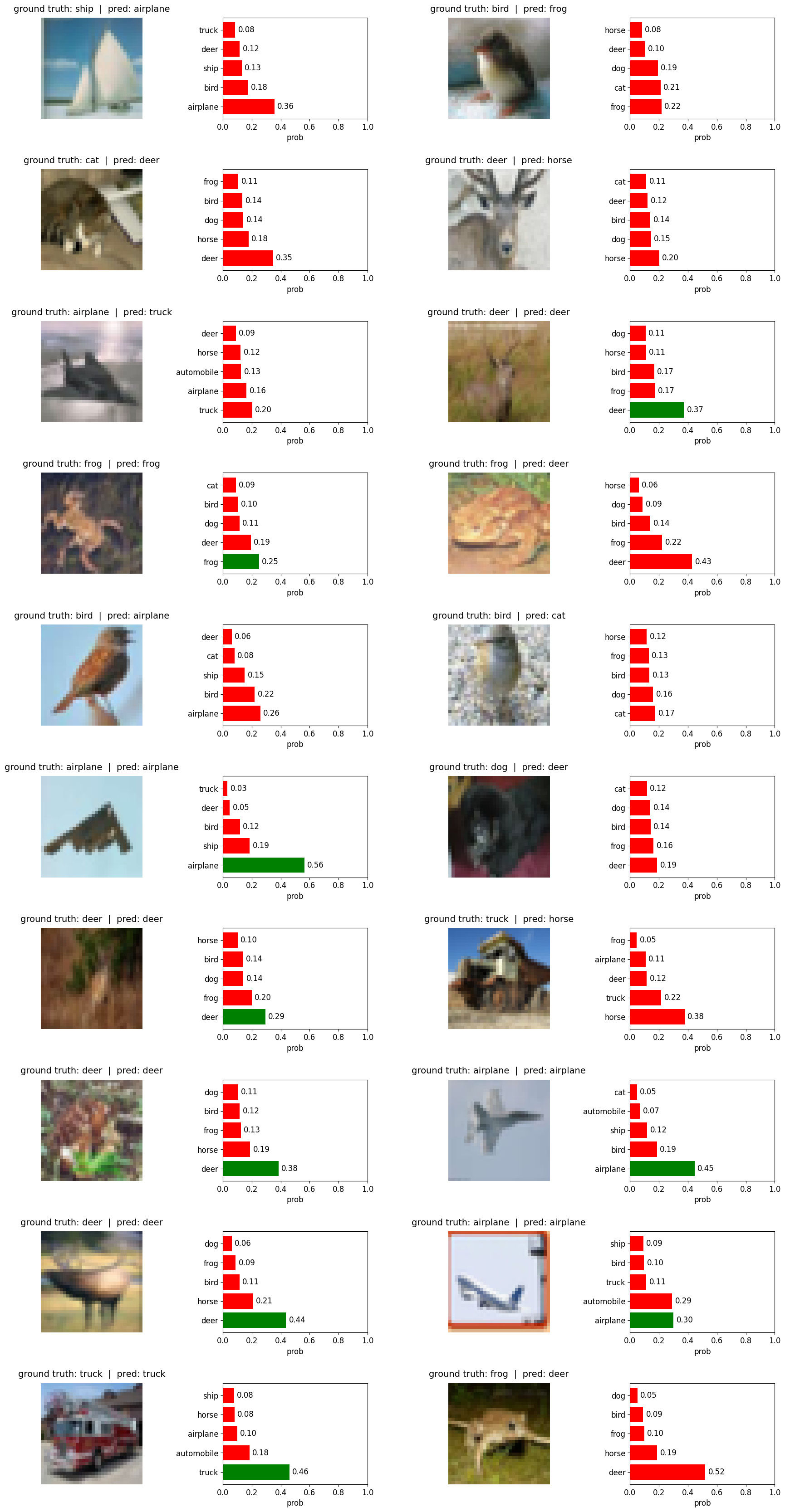
test after 1 epoch#
test_random_200()
==> Test accuracy on random 200 from test set: 0.345
/var/folders/hr/kvb_nv256v958_chgsmxrsdm0000gn/T/ipykernel_65363/912593212.py:97: UserWarning: This figure includes Axes that are not compatible with tight_layout, so results might be incorrect.
  plt.tight_layout()
Running it for remainder of epoch (total 15) and perform the test again on the same sample…#
run_one_epoch()
run_one_epoch()
run_one_epoch()
run_one_epoch()
run_one_epoch()
run_one_epoch()
run_one_epoch()
run_one_epoch()
run_one_epoch()
run_one_epoch()
run_one_epoch()
run_one_epoch()
run_one_epoch()
run_one_epoch()
# run the test again...
test_random_200()
Train Epoch 2/15 - Time: 17.07s
==>Training Loss: 1.5760 - Training Accuracy: 43.49% - Test Loss: 1.5136 - Test Accuracy: 46.31%
Train Epoch 3/15 - Time: 16.79s
==>Training Loss: 1.4043 - Training Accuracy: 49.82% - Test Loss: 1.3750 - Test Accuracy: 50.47%
Train Epoch 4/15 - Time: 16.66s
==>Training Loss: 1.2846 - Training Accuracy: 54.38% - Test Loss: 1.2802 - Test Accuracy: 55.78%
Train Epoch 5/15 - Time: 16.41s
==>Training Loss: 1.1896 - Training Accuracy: 58.25% - Test Loss: 1.1818 - Test Accuracy: 58.91%
Train Epoch 6/15 - Time: 16.45s
==>Training Loss: 1.1210 - Training Accuracy: 60.96% - Test Loss: 1.1142 - Test Accuracy: 61.12%
Train Epoch 7/15 - Time: 16.74s
==>Training Loss: 1.0610 - Training Accuracy: 63.04% - Test Loss: 1.1105 - Test Accuracy: 60.73%
Train Epoch 8/15 - Time: 17.31s
==>Training Loss: 1.0010 - Training Accuracy: 65.05% - Test Loss: 1.0576 - Test Accuracy: 63.30%
Train Epoch 9/15 - Time: 17.17s
==>Training Loss: 0.9803 - Training Accuracy: 65.75% - Test Loss: 1.0764 - Test Accuracy: 62.95%
Train Epoch 10/15 - Time: 17.36s
==>Training Loss: 0.9430 - Training Accuracy: 67.00% - Test Loss: 1.0451 - Test Accuracy: 63.28%
Train Epoch 11/15 - Time: 17.59s
==>Training Loss: 0.9145 - Training Accuracy: 68.01% - Test Loss: 1.0260 - Test Accuracy: 64.41%
Train Epoch 12/15 - Time: 17.80s
==>Training Loss: 0.8862 - Training Accuracy: 69.03% - Test Loss: 1.0014 - Test Accuracy: 65.11%
Train Epoch 13/15 - Time: 17.41s
==>Training Loss: 0.8690 - Training Accuracy: 69.55% - Test Loss: 0.9655 - Test Accuracy: 66.57%
Train Epoch 14/15 - Time: 17.95s
==>Training Loss: 0.8443 - Training Accuracy: 70.29% - Test Loss: 0.9700 - Test Accuracy: 66.73%
Train Epoch 15/15 - Time: 18.46s
==>Training Loss: 0.8255 - Training Accuracy: 71.11% - Test Loss: 0.9726 - Test Accuracy: 67.02%

==> Test accuracy on random 200 from test set: 0.675
/var/folders/hr/kvb_nv256v958_chgsmxrsdm0000gn/T/ipykernel_65363/912593212.py:97: UserWarning: This figure includes Axes that are not compatible with tight_layout, so results might be incorrect.
  plt.tight_layout()
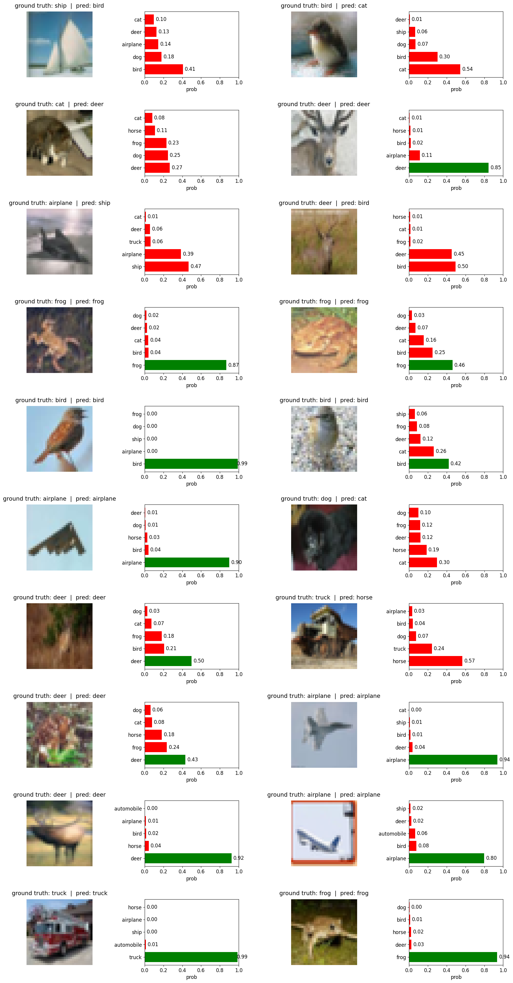
Note ⚠️: 15 epoch’s are too less and the model was still learning… the accuracy after 15 epochs is not the best but its just to show the progress and improvements…
Visualize Conv Layers#
we will create a simple hook to save the activations output. This will be registered as forward hooks with each layer. Since activations is a simple object, it will be overwritten for each input tensor during training
activations = {}

def save_activation(name):
    def hook(module, inp, out):
        # out is (B,C,H,W); store only first sample -> (C,H,W)
        activations[name] = {"act": out[0].detach().cpu()}
    return hook
we will name the layers to store the activations outputs… we will use this later for visualizations
META = "__meta__"
CONV1 = "conv1 (32x32x16)"
RELU1 = "relu1 (32x32x16)"
POOL1 = "pool1 (16x16x16)"
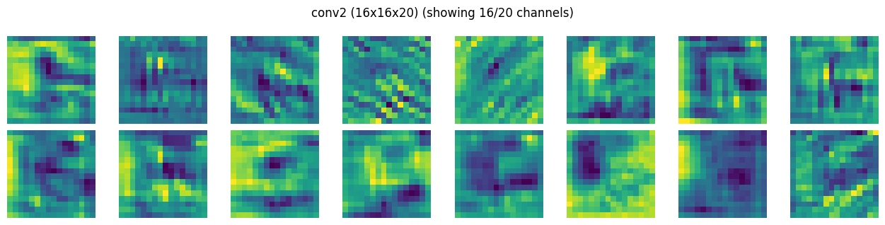
CONV2 = "conv2 (16x16x20)"
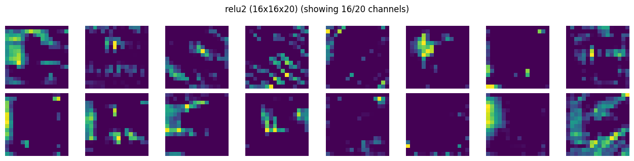
RELU2 = "relu2 (16x16x20)"
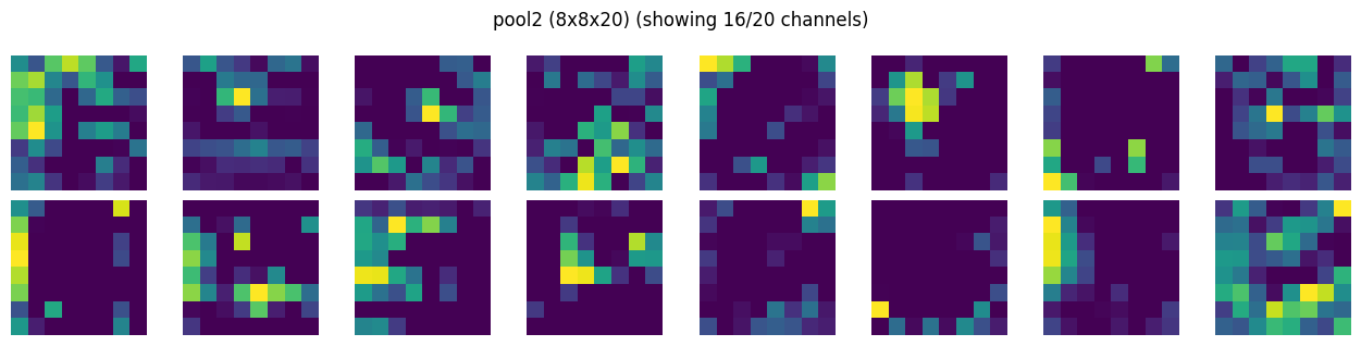
POOL2 = "pool2 (8x8x20)"
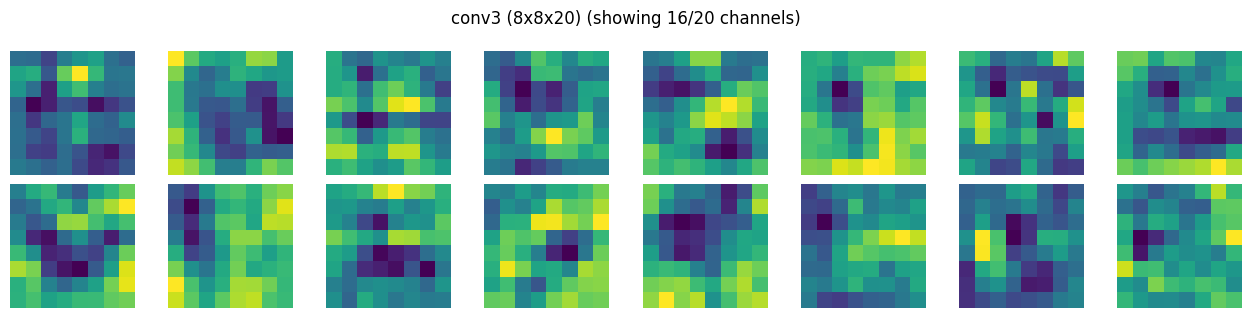
CONV3 = "conv3 (8x8x20)"
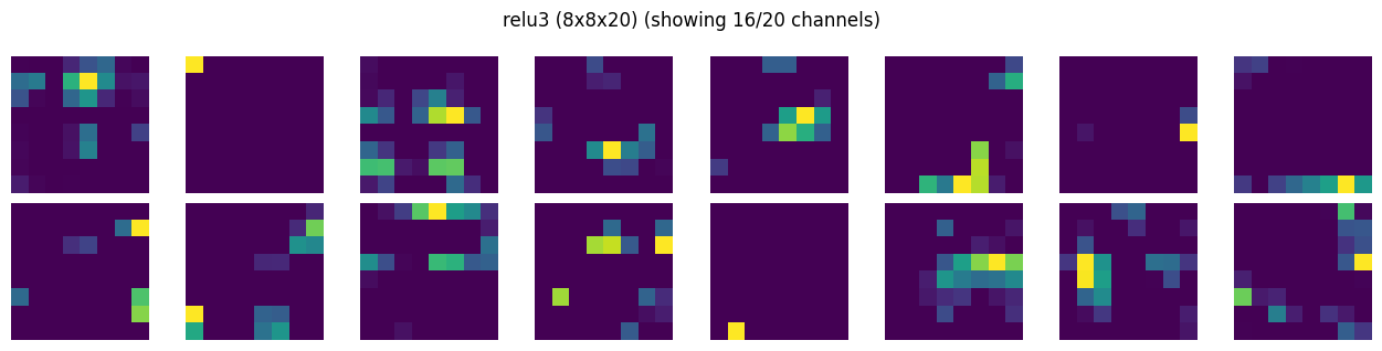
RELU3 = "relu3 (8x8x20)"
POOL3 = "pool3 (4x4x20)"
Capture activations with forward hooks#
we will use this for visualizations
hooks = []
hooks.append(model.conv1.register_forward_hook(save_activation(CONV1)))
hooks.append(model.relu1.register_forward_hook(save_activation(RELU1)))
hooks.append(model.pool1.register_forward_hook(save_activation(POOL1)))
hooks.append(model.conv2.register_forward_hook(save_activation(CONV2)))
hooks.append(model.relu2.register_forward_hook(save_activation(RELU2)))
hooks.append(model.pool2.register_forward_hook(save_activation(POOL2)))
hooks.append(model.conv3.register_forward_hook(save_activation(CONV3)))
hooks.append(model.relu3.register_forward_hook(save_activation(RELU3)))
hooks.append(model.pool3.register_forward_hook(save_activation(POOL3)))
… single forward pass so that we capture the activation maps
sample = 4667
activations.clear()

# Build a (1,3,32,32) tensor
x1 = torch.from_numpy(x_batch1[sample]).float() / 255.0          # (32,32,3)
x1 = x1.permute(2,0,1).unsqueeze(0).to(device)                   # (1,3,32,32)

# Store meta (optional but nice)
activations[META] = {
    "sample": sample,
    "y": int(y_batch1[sample]),
    "x": x1[0].detach().cpu(),   # (3,32,32)
}

model.eval()
with torch.no_grad():
    logits = model(x1)   # hooks would fire here...
    prob = torch.softmax(logits, dim=1)
tensor([[-0.6300,  7.2815, -2.9838, -2.7433, -4.4819, -3.8679, -3.6393, -5.6147,
          2.9944, 11.9750]])
import matplotlib.pyplot as plt

def show_activation_maps(activation_maps, title, max_channels=16, cols=8):
    t = activation_maps.detach().cpu()
    C, H, W = t.shape
    n = min(C, max_channels)
    rows = (n + cols - 1) // cols

    plt.figure(figsize=(cols*1.6, rows*1.6))
    for i in range(n):
        ax = plt.subplot(rows, cols, i+1)
        ax.imshow(t[i].numpy())
        ax.axis("off")
    plt.suptitle(f"{title} (showing {n}/{C} channels)")
    plt.tight_layout()
    plt.show()
img = activations[META]["x"].permute(1,2,0).numpy()
plt.imshow(img)
plt.title(f"label: {class_names[activations[META]['y']]} ({activations[META]['y']})")
plt.show()
probs = prob[0].cpu().numpy()

print(f"--- Predictions for Sample {activations[META]['sample']} ---")
for i, p in enumerate(probs):
    name = class_names[i]
    percentage = p * 100
    print(f"{name:10}: {percentage:>6.2f}%")
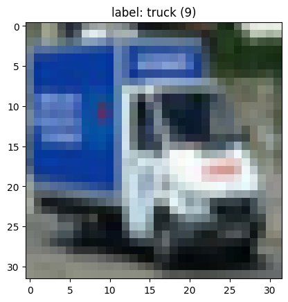
--- Predictions for Sample 4667 ---
airplane  :   0.00%
automobile:   0.91%
bird      :   0.00%
cat       :   0.00%
deer      :   0.00%
dog       :   0.00%
frog      :   0.00%
horse     :   0.00%
ship      :   0.01%
truck     :  99.08%
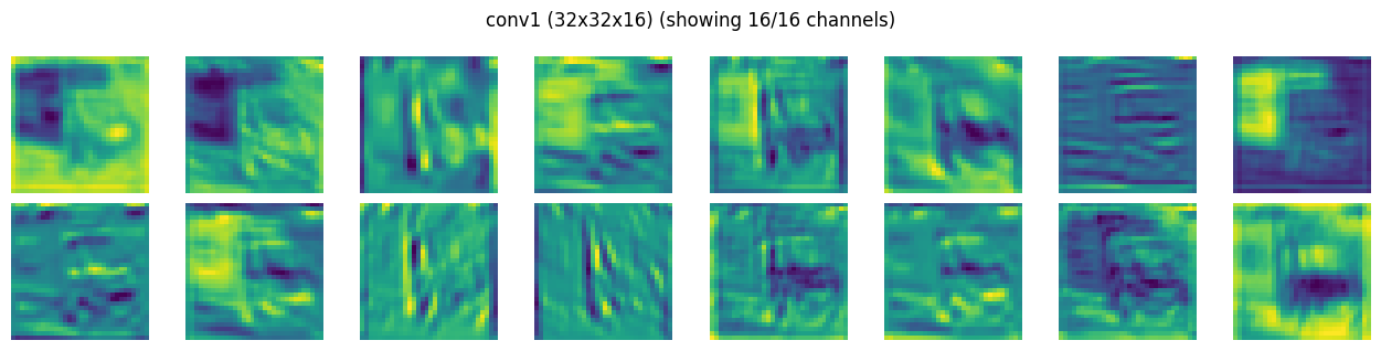
# show feature maps per layer
show_activation_maps(activations[CONV1]["act"], CONV1)
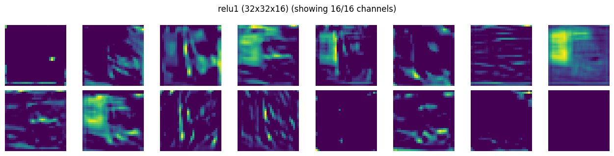
show_activation_maps(activations[RELU1]["act"], RELU1)
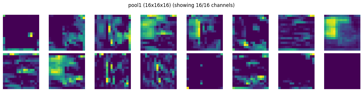
show_activation_maps(activations[POOL1]["act"], POOL1)
show_activation_maps(activations[CONV2]["act"], CONV2)
show_activation_maps(activations[RELU2]["act"], RELU2)
show_activation_maps(activations[POOL2]["act"], POOL2)
show_activation_maps(activations[CONV3]["act"], CONV3)
show_activation_maps(activations[RELU3]["act"], RELU3)
show_activation_maps(activations[POOL3]["act"], POOL3)

Just for science#
this is how the kernal or filter looks like post training for CONV1
def show_conv_filters(weight: torch.Tensor, max_filters=16, cols=8, title=""):
    W = weight.detach().cpu()
    out_ch, in_ch, kH, kW = W.shape
    n = min(out_ch, max_filters)
    rows = (n + cols - 1) // cols

    plt.figure(figsize=(cols * 1.6, rows * 1.6))
    for i in range(n):
        ax = plt.subplot(rows, cols, i + 1)
        w = W[i]

        if in_ch == 3:
            img = w.permute(1,2,0).numpy()
            img = (img - img.min()) / (img.max() - img.min() + 1e-8)
            ax.imshow(img)
        else:
            ax.imshow(w[0].numpy())
        ax.axis("off")

    plt.suptitle(title)
    plt.tight_layout()
    plt.show()

show_conv_filters(model.conv1.weight, title="conv1 16x filters (post-training)")
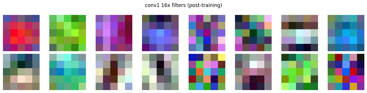
note: the darker and lighter green with blacks in conv1 output is a visualization artifact (normalized for plotting) and is hiding the positive and negative values of tensors. The respecitve relu1 layer (see the first activation map) might give an impression that its killing majority of tensors, but imagine smallest value to be black, largest value to be yellow/lightgreen, and rest (negatives) are scaled in between…