◉ DINOv3#
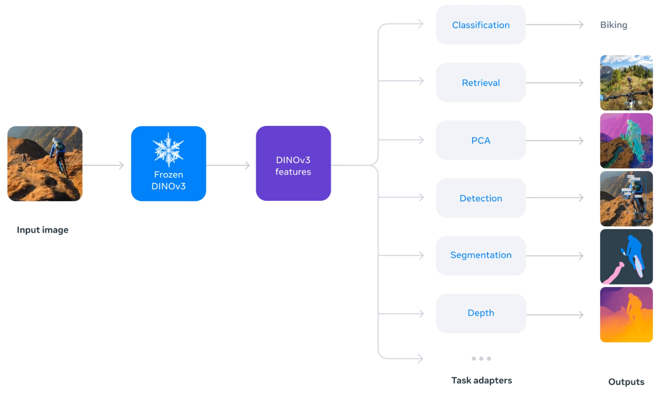
DINOv3 is a vision foundational model and can be tuned to perform various vision task. I just wanted to understand how Meta did the text alignment with dino.txt for text-to-image retrieval task…
![]()
downloaded the checkpoints from here…
from dinov3.hub.dinotxt import dinov3_vitl16_dinotxt_tet1280d20h24l
model, tokenizer = dinov3_vitl16_dinotxt_tet1280d20h24l(
    weights="../models/dinov3_vitl16_dinotxt_vision_head_and_text_encoder-a442d8f5.pth",
    backbone_weights="../models/dinov3_vitl16_pretrain_lvd1689m-8aa4cbdd.pth",
    bpe_path_or_url="../models/bpe_simple_vocab_16e6.txt.gz"
)
model
DINOTxt(
  (visual_model): VisionTower(
    (backbone): DinoVisionTransformer(
      (patch_embed): PatchEmbed(
        (proj): Conv2d(3, 1024, kernel_size=(16, 16), stride=(16, 16))
        (norm): Identity()
      )
      (rope_embed): RopePositionEmbedding()
      (blocks): ModuleList(
        (0-23): 24 x SelfAttentionBlock(
          (norm1): LayerNorm((1024,), eps=1e-05, elementwise_affine=True)
          (attn): SelfAttention(
            (qkv): LinearKMaskedBias(in_features=1024, out_features=3072, bias=True)
            (attn_drop): Dropout(p=0.0, inplace=False)
            (proj): Linear(in_features=1024, out_features=1024, bias=True)
            (proj_drop): Dropout(p=0.0, inplace=False)
          )
          (ls1): LayerScale()
          (norm2): LayerNorm((1024,), eps=1e-05, elementwise_affine=True)
          (mlp): Mlp(
            (fc1): Linear(in_features=1024, out_features=4096, bias=True)
            (act): GELU(approximate='none')
            (fc2): Linear(in_features=4096, out_features=1024, bias=True)
            (drop): Dropout(p=0.0, inplace=False)
          )
          (ls2): LayerScale()
        )
      )
      (norm): LayerNorm((1024,), eps=1e-05, elementwise_affine=True)
      (head): Identity()
    )
    (head): VisionHead(
      (ln_final): LayerNorm((1024,), eps=1e-05, elementwise_affine=True)
      (blocks): ModuleList(
        (0-1): 2 x SelfAttentionBlock(
          (norm1): LayerNorm((1024,), eps=1e-05, elementwise_affine=True)
          (attn): SelfAttention(
            (qkv): Linear(in_features=1024, out_features=3072, bias=False)
            (attn_drop): Dropout(p=0.0, inplace=False)
            (proj): Linear(in_features=1024, out_features=1024, bias=True)
            (proj_drop): Dropout(p=0.0, inplace=False)
          )
          (ls1): LayerScale()
          (norm2): LayerNorm((1024,), eps=1e-05, elementwise_affine=True)
          (mlp): SwiGLUFFN(
            (w1): Linear(in_features=1024, out_features=2752, bias=True)
            (w2): Linear(in_features=1024, out_features=2752, bias=True)
            (w3): Linear(in_features=2752, out_features=1024, bias=True)
          )
          (ls2): LayerScale()
        )
      )
      (linear_projection): Identity()
    )
  )
  (text_model): TextTower(
    (backbone): TextTransformer(
      (token_embedding): Embedding(49408, 1280)
      (dropout): Dropout(p=0.0, inplace=False)
      (blocks): ModuleList(
        (0-23): 24 x CausalSelfAttentionBlock(
          (ls1): Identity()
          (attention_norm): LayerNorm((1280,), eps=1e-05, elementwise_affine=True)
          (attention): CausalSelfAttention(
            (qkv): Linear(in_features=1280, out_features=3840, bias=False)
            (proj): Linear(in_features=1280, out_features=1280, bias=True)
            (proj_drop): Dropout(p=0.0, inplace=False)
          )
          (ffn_norm): LayerNorm((1280,), eps=1e-05, elementwise_affine=True)
          (feed_forward): Mlp(
            (fc1): Linear(in_features=1280, out_features=5120, bias=True)
            (act): GELU(approximate='none')
            (fc2): Linear(in_features=5120, out_features=1280, bias=True)
            (drop): Dropout(p=0.0, inplace=False)
          )
          (ls2): Identity()
        )
      )
      (ln_final): LayerNorm((1280,), eps=1e-05, elementwise_affine=True)
    )
    (head): TextHead(
      (ln_final): Identity()
      (blocks): ModuleList(
        (0): Identity()
      )
      (linear_projection): Linear(in_features=1280, out_features=2048, bias=False)
    )
  )
)
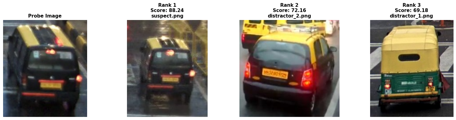
DinoV3 ViT-L Similarity Search#
Search a probe image in the presence of distractors. Reason why we would need a dedicated ReID model
import os
from pathlib import Path
import matplotlib.pyplot as plt
from PIL import Image
import torch
from dinov3.data.transforms import make_classification_eval_transform
import torch.nn.functional as F

image_preprocess = make_classification_eval_transform()
softmax_temperature = 100.0

image_dir = Path("../models/images/")
image_paths = list(image_dir.glob("*.jpg")) + list(image_dir.glob("*.png")) + list(image_dir.glob("*.jpeg"))
print(f"Found {len(image_paths)} images")

images_pil = [Image.open(p).convert("RGB") for p in image_paths]
image_tensors = torch.stack([image_preprocess(img) for img in images_pil]).cuda()

with torch.autocast('cuda', dtype=torch.float):
    with torch.no_grad():
        all_image_features = model.encode_image(image_tensors)
        all_image_features /= all_image_features.norm(dim=-1, keepdim=True)

print(f"Embedded {len(image_paths)} images → shape: {all_image_features.shape}")
Found 14 images
Embedded 14 images → shape: torch.Size([14, 2048])
probe = Image.open("../models/probe/probe.png").convert("RGB")
probe_tensor = torch.stack([image_preprocess(probe)], dim=0).cuda()

with torch.autocast('cuda', dtype=torch.float):
    with torch.no_grad():
        probe_features = model.encode_image(probe_tensor)
probe_features /= probe_features.norm(dim=-1, keepdim=True)

similarity_matrix = (probe_features @ all_image_features.T).cpu().float().numpy()
similarity_scores = similarity_matrix[0] * 100.0
import matplotlib.pyplot as plt

top_k = 3
top_indices = similarity_scores.argsort()[::-1][:top_k]
top_scores = similarity_scores[top_indices]


print(f"Top {top_k} matches for input probe image")

fig, axes = plt.subplots(1, top_k + 1, figsize=(4*(top_k + 1), 4))

axes[0].imshow(probe)
axes[0].set_title("Probe Image", fontsize=11, fontweight='bold')
axes[0].axis('off')

for rank, (ax, img_idx) in enumerate(zip(axes[1:], top_indices)):
    ax.imshow(images_pil[img_idx])
    ax.set_title(f"Rank {rank+1}\nScore: {top_scores[rank]:.2f}\n{image_paths[img_idx].name}",
                 fontsize=11, fontweight='bold')
    ax.axis('off')

plt.tight_layout()
plt.show()
Top 3 matches for input probe image
Zero-shot classification on ImageNet1k#
Its hard to get access to ImageNet1K without an research/institution backing… will use Imagenette dataset instead that comes with 10 class…
n01440764 (tench)
n02102040 (English springer)
n02979186 (cassette player)
n03000684 (chain saw)
n03028079 (church)
n03394916 (French horn)
n03417042 (garbage truck)
n03425413 (gas pump)
n03445777 (golf ball)
n03888257 (parachute)
imagenette_class_names = ["tench", "English Springer Spaniel", "cassette player",
                           "chainsaw", "church", "French horn", "garbage truck",
                           "gas pump", "golf ball", "parachute"]
# The following comes from here: https://github.com/mlfoundations/open_clip/blob/main/src/open_clip/zero_shot_metadata.py
# Original reference: https://github.com/openai/CLIP/blob/main/notebooks/Prompt_Engineering_for_ImageNet.ipynb
openai_imagenet_templates = (
    lambda c: f"a bad photo of a {c}.",
    lambda c: f"a photo of many {c}.",
    lambda c: f"a sculpture of a {c}.",
    lambda c: f"a photo of the hard to see {c}.",
    lambda c: f"a low resolution photo of the {c}.",
    lambda c: f"a rendering of a {c}.",
    lambda c: f"graffiti of a {c}.",
    lambda c: f"a bad photo of the {c}.",
    lambda c: f"a cropped photo of the {c}.",
    lambda c: f"a tattoo of a {c}.",
    lambda c: f"the embroidered {c}.",
    lambda c: f"a photo of a hard to see {c}.",
    lambda c: f"a bright photo of a {c}.",
    lambda c: f"a photo of a clean {c}.",
    lambda c: f"a photo of a dirty {c}.",
    lambda c: f"a dark photo of the {c}.",
    lambda c: f"a drawing of a {c}.",
    lambda c: f"a photo of my {c}.",
    lambda c: f"the plastic {c}.",
    lambda c: f"a photo of the cool {c}.",
    lambda c: f"a close-up photo of a {c}.",
    lambda c: f"a black and white photo of the {c}.",
    lambda c: f"a painting of the {c}.",
    lambda c: f"a painting of a {c}.",
    lambda c: f"a pixelated photo of the {c}.",
    lambda c: f"a sculpture of the {c}.",
    lambda c: f"a bright photo of the {c}.",
    lambda c: f"a cropped photo of a {c}.",
    lambda c: f"a plastic {c}.",
    lambda c: f"a photo of the dirty {c}.",
    lambda c: f"a jpeg corrupted photo of a {c}.",
    lambda c: f"a blurry photo of the {c}.",
    lambda c: f"a photo of the {c}.",
    lambda c: f"a good photo of the {c}.",
    lambda c: f"a rendering of the {c}.",
    lambda c: f"a {c} in a video game.",
    lambda c: f"a photo of one {c}.",
    lambda c: f"a doodle of a {c}.",
    lambda c: f"a close-up photo of the {c}.",
    lambda c: f"a photo of a {c}.",
    lambda c: f"the origami {c}.",
    lambda c: f"the {c} in a video game.",
    lambda c: f"a sketch of a {c}.",
    lambda c: f"a doodle of the {c}.",
    lambda c: f"a origami {c}.",
    lambda c: f"a low resolution photo of a {c}.",
    lambda c: f"the toy {c}.",
    lambda c: f"a rendition of the {c}.",
    lambda c: f"a photo of the clean {c}.",
    lambda c: f"a photo of a large {c}.",
    lambda c: f"a rendition of a {c}.",
    lambda c: f"a photo of a nice {c}.",
    lambda c: f"a photo of a weird {c}.",
    lambda c: f"a blurry photo of a {c}.",
    lambda c: f"a cartoon {c}.",
    lambda c: f"art of a {c}.",
    lambda c: f"a sketch of the {c}.",
    lambda c: f"a embroidered {c}.",
    lambda c: f"a pixelated photo of a {c}.",
    lambda c: f"itap of the {c}.",
    lambda c: f"a jpeg corrupted photo of the {c}.",
    lambda c: f"a good photo of a {c}.",
    lambda c: f"a plushie {c}.",
    lambda c: f"a photo of the nice {c}.",
    lambda c: f"a photo of the small {c}.",
    lambda c: f"a photo of the weird {c}.",
    lambda c: f"the cartoon {c}.",
    lambda c: f"art of the {c}.",
    lambda c: f"a drawing of the {c}.",
    lambda c: f"a photo of the large {c}.",
    lambda c: f"a black and white photo of a {c}.",
    lambda c: f"the plushie {c}.",
    lambda c: f"a dark photo of a {c}.",
    lambda c: f"itap of a {c}.",
    lambda c: f"graffiti of the {c}.",
    lambda c: f"a toy {c}.",
    lambda c: f"itap of my {c}.",
    lambda c: f"a photo of a cool {c}.",
    lambda c: f"a photo of a small {c}.",
    lambda c: f"a tattoo of the {c}.",
)
from torchvision.datasets import ImageFolder
from dinov3.data.transforms import make_classification_eval_transform

image_preprocess = make_classification_eval_transform(resize_size=512, crop_size=512)
imagenet_val_root_dir = "../models/imagenette2/val/"
val_dataset = ImageFolder(imagenet_val_root_dir, image_preprocess)
model = model.eval().cuda()

for idx, class_name in enumerate(val_dataset.class_to_idx):
    print("id:", idx, "ImageNet Class:", class_name, "Name:", imagenette_class_names[idx])
id: 0 ImageNet Class: n01440764 Name: tench
id: 1 ImageNet Class: n02102040 Name: English Springer Spaniel
id: 2 ImageNet Class: n02979186 Name: cassette player
id: 3 ImageNet Class: n03000684 Name: chainsaw
id: 4 ImageNet Class: n03028079 Name: church
id: 5 ImageNet Class: n03394916 Name: French horn
id: 6 ImageNet Class: n03417042 Name: garbage truck
id: 7 ImageNet Class: n03425413 Name: gas pump
id: 8 ImageNet Class: n03445777 Name: golf ball
id: 9 ImageNet Class: n03888257 Name: parachute
Note that the Dataloder have absolutely no clue of what a tench or chainsaw is, it was only trained on the class label i.e. its id. There is no connection between imagenette_class_names (which is meant only for readability) and how DataLoader loads the subfolders inside /val - I had to explicitly map the folders to its respective class for presentation purpose…
def zeroshot_classifier(classnames, templates, tokenizer):
    with torch.no_grad():
        zeroshot_weights = []
        for classname in classnames:
            texts = [template(classname) for template in templates] #format with class
            texts = tokenizer.tokenize(texts).cuda() #tokenize
            class_embeddings = model.encode_text(texts) #embed with text encoder
            class_embeddings /= class_embeddings.norm(dim=-1, keepdim=True)
            class_embedding = class_embeddings.mean(dim=0)
            class_embedding /= class_embedding.norm()
            zeroshot_weights.append(class_embedding)
        zeroshot_weights = torch.stack(zeroshot_weights, dim=1).cuda()
    return zeroshot_weights
zeroshot_weights = zeroshot_classifier(imagenette_class_names, openai_imagenet_templates, tokenizer)
def accuracy(output, target, topk=(1,), should_print=False, scale=100.):
    pred = output.topk(max(topk), 1, True, True)[1].t()
    correct = pred.eq(target.view(1, -1).expand_as(pred))
    if should_print:
        top_vals, top_idxs = output[0].topk(max(topk))
        raw_scores = top_vals / scale  # Remove scaling to get cosine similarity

        print(f"\n{'='*60}")
        for i, k in enumerate(range(max(topk))):
            class_name = imagenette_class_names[top_idxs[k].item()]
            print(f"Top-{k+1}: {class_name:25s} | Logit: {top_vals[k]:.2f} | Cosine: {raw_scores[k]:.4f}")
        print(f"Ground truth: {imagenette_class_names[target[0].item()]}")
        print(f"{'='*60}")
    return [correct[:k].reshape(-1).sum(0, keepdim=True) for k in topk]
images = []
class_ids = []
batch_size = 64
num_workers = 8
top1, top5, n = 0., 0., 0.
print_every = 10
val_loader = torch.utils.data.DataLoader(val_dataset, batch_size=batch_size, shuffle=False, num_workers=num_workers, pin_memory=True)
for idx, (images, targets) in enumerate(val_loader):
    with torch.autocast('cuda', dtype=torch.float):
        with torch.no_grad():
            image_features = model.encode_image(images.cuda())
            image_features /= image_features.norm(dim=-1, keepdim=True)
            logits = 100. * image_features @ zeroshot_weights
            acc1, acc5 = accuracy(logits, targets.cuda(), topk=(1, 5), should_print=True if idx % print_every == 0 else False)
            top1 += acc1
            top5 += acc5
            n += len(images)
    images = []
    class_ids = []
    if idx % print_every == 0:
        print(f"Running Top-1: {(top1.item() / n) * 100:.2f}%, Top-5: {(top5.item() / n) * 100:.2f}% after {n} samples")
top1 = (top1.item() / n) * 100
top5 = (top5.item() / n) * 100

print(f"{'-'*30}")
print(f"Final Top-1 accuracy: {top1:.2f}%")
print(f"Final Top-5 accuracy: {top5:.2f}%")
============================================================
Top-1: tench                     | Logit: 26.64 | Cosine: 0.2664
Top-2: chainsaw                  | Logit: 6.50 | Cosine: 0.0650
Top-3: parachute                 | Logit: 6.26 | Cosine: 0.0626
Top-4: French horn               | Logit: 5.34 | Cosine: 0.0534
Top-5: gas pump                  | Logit: 4.63 | Cosine: 0.0463
Ground truth: tench
============================================================
Running Top-1: 98.44%, Top-5: 98.44% after 64.0 samples

============================================================
Top-1: English Springer Spaniel  | Logit: 17.58 | Cosine: 0.1758
Top-2: church                    | Logit: 6.15 | Cosine: 0.0615
Top-3: garbage truck             | Logit: 6.07 | Cosine: 0.0607
Top-4: golf ball                 | Logit: 5.63 | Cosine: 0.0563
Top-5: gas pump                  | Logit: 5.14 | Cosine: 0.0514
Ground truth: English Springer Spaniel
============================================================
Running Top-1: 99.86%, Top-5: 99.86% after 704.0 samples

============================================================
Top-1: chainsaw                  | Logit: 15.50 | Cosine: 0.1550
Top-2: gas pump                  | Logit: 6.71 | Cosine: 0.0671
Top-3: church                    | Logit: 4.50 | Cosine: 0.0450
Top-4: garbage truck             | Logit: 3.07 | Cosine: 0.0307
Top-5: cassette player           | Logit: 2.71 | Cosine: 0.0271
Ground truth: chainsaw
============================================================
Running Top-1: 99.78%, Top-5: 99.85% after 1344.0 samples

============================================================
Top-1: church                    | Logit: 15.55 | Cosine: 0.1555
Top-2: chainsaw                  | Logit: 5.65 | Cosine: 0.0565
Top-3: English Springer Spaniel  | Logit: 5.63 | Cosine: 0.0563
Top-4: French horn               | Logit: 4.85 | Cosine: 0.0485
Top-5: parachute                 | Logit: 3.83 | Cosine: 0.0383
Ground truth: church
============================================================
Running Top-1: 99.80%, Top-5: 99.90% after 1984.0 samples

============================================================
Top-1: garbage truck             | Logit: 24.05 | Cosine: 0.2405
Top-2: cassette player           | Logit: 9.18 | Cosine: 0.0918
Top-3: church                    | Logit: 8.74 | Cosine: 0.0874
Top-4: gas pump                  | Logit: 8.13 | Cosine: 0.0813
Top-5: golf ball                 | Logit: 7.70 | Cosine: 0.0770
Ground truth: garbage truck
============================================================
Running Top-1: 99.85%, Top-5: 99.92% after 2624.0 samples

============================================================
Top-1: golf ball                 | Logit: 15.93 | Cosine: 0.1593
Top-2: gas pump                  | Logit: 3.92 | Cosine: 0.0392
Top-3: parachute                 | Logit: 2.53 | Cosine: 0.0253
Top-4: English Springer Spaniel  | Logit: 2.26 | Cosine: 0.0226
Top-5: chainsaw                  | Logit: 1.60 | Cosine: 0.0160
Ground truth: golf ball
============================================================
Running Top-1: 99.85%, Top-5: 99.94% after 3264.0 samples

============================================================
Top-1: parachute                 | Logit: 20.56 | Cosine: 0.2056
Top-2: French horn               | Logit: 6.11 | Cosine: 0.0611
Top-3: golf ball                 | Logit: 5.78 | Cosine: 0.0578
Top-4: church                    | Logit: 5.45 | Cosine: 0.0545
Top-5: gas pump                  | Logit: 4.58 | Cosine: 0.0458
Ground truth: parachute
============================================================
Running Top-1: 99.87%, Top-5: 99.95% after 3904.0 samples
------------------------------
Final Top-1 accuracy: 99.87%
Final Top-5 accuracy: 99.95%
Why the cosine numbers look “low”???#
just a bit of theory first… For two normalized embeddings (x) and (y),
where:
(\(\theta\)) is the angle between the two vectors
both vectors have length 1
cosine depends only on direction, not magnitude
so…
angle (\(0^\circ\)) == cosine (1.0) == exactly same direction
angle (\(90^\circ\)) == cosine (0.0) == orthogonal
angle (\(180^\circ\)) == cosine (-1.0) == opposite direction
now the angle is calculated as
e.g. $\( \theta = \arccos(\text{0.20}) = 78.5° \)$
In high-D 78.5° is still quite meaningful
Understand modality gap in mixed modality embedding space#
Text and images can be in the same 2048-D space, but that does not mean they are uniformly intermingled. In aligned vision-language models, the goal is that matching image/text pairs have higher cosine similarity than non-matching pairs. That still allows a modality gap: image embeddings may occupy one region/structure of the space and text embeddings another, even though they are comparable with cosine similarity. Understand that the intra-modal distances is usually smaller than inter-modal distances, meaning image-image and text-text neighborhoods may still be tighter than image-text neighborhoods. paper link
Calibration to calucate confidence (sigmoid) from Cosine#
Cosine similarity = geometry of two embedding vectors
Sigmoid calibration = how we map that geometric score into a human-friendly confidence-like number
Threshold is the cosine value where sigmoid outputs 0.5. With threshold=0.10, temp=20:
Cosine Score |
Confidence |
|---|---|
0.27 (tench) |
97% |
0.24 (garbage truck) |
94% |
0.20 (parachute) |
88% |
0.18 (springer) |
82% |
0.155 (church/chainsaw) |
73% |
trying a few values…
threshold |
temp |
Effect |
|---|---|---|
0.10 |
20 |
Church=73%, Tench=97% |
0.08 |
25 |
Church=84%, Tench=99% — more confident overall |
threshold = 0.08
temperature = 25
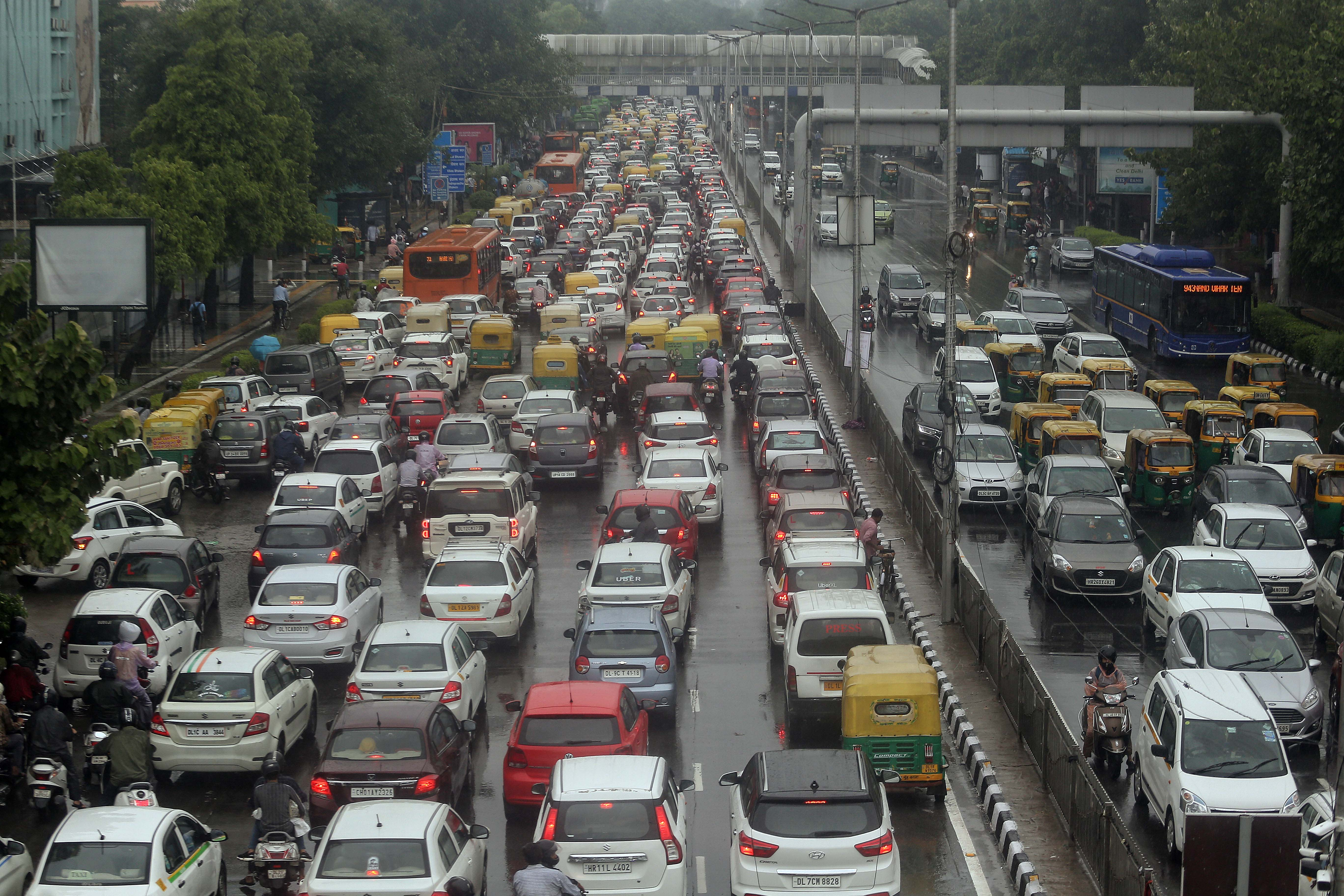
Query on on single image#
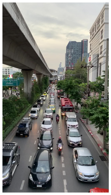
“traffic jam on a wet road with many vehicles lane splitting”
from PIL import Image

img_pil = Image.open("../models/images/crowd.jpg").convert("RGB")
display(img_pil)
import torch
from dinov3.data.transforms import make_classification_eval_transform
import torch.nn.functional as F

image_preprocess = make_classification_eval_transform()
image_tensor = torch.stack([image_preprocess(img_pil)], dim=0).cuda()
texts = ["traffic jam on a wet road with many vehicles lane splitting"]
tokenized_texts_tensor = tokenizer.tokenize(texts).cuda()
model = model.cuda()
with torch.autocast('cuda', dtype=torch.float):
    with torch.no_grad():
        image_features = model.encode_image(image_tensor)
        text_features = model.encode_text(tokenized_texts_tensor)
image_features /= image_features.norm(dim=-1, keepdim=True)
text_features /= text_features.norm(dim=-1, keepdim=True)
similarity = (
    text_features.cpu().float().numpy() @ image_features.cpu().float().numpy().T
)
print(f"Score: {similarity[0][0] * 100:.2f}")
Score: 19.76
Testing multiple text queries on our images embeddings#
import os
from pathlib import Path
import matplotlib.pyplot as plt

def test_text_to_image_retrieval(image_dir, text_queries):

    softmax_temperature = 100.0

    image_paths = list(image_dir.glob("*.jpg")) + list(image_dir.glob("*.png")) + list(image_dir.glob("*.jpeg"))
    print(f"Found {len(image_paths)} images")

    images_pil = [Image.open(p).convert("RGB") for p in image_paths]
    image_tensors = torch.stack([image_preprocess(img) for img in images_pil]).cuda()

    with torch.autocast('cuda', dtype=torch.float):
        with torch.no_grad():
            all_image_features = model.encode_image(image_tensors)
            all_image_features /= all_image_features.norm(dim=-1, keepdim=True)

    print(f"Embedded {len(image_paths)} images → shape: {all_image_features.shape}")

    tokenized_queries = tokenizer.tokenize(text_queries).cuda()
    with torch.autocast('cuda', dtype=torch.float):
        with torch.no_grad():
            query_features = model.encode_text(tokenized_queries)
            query_features /= query_features.norm(dim=-1, keepdim=True)

    similarity_matrix = (query_features @ all_image_features.T).cpu().float().numpy()

    top_k = 3

    for query_idx, query_text in enumerate(text_queries):
        scores = similarity_matrix[query_idx]

        # Compute probabilities across ALL images first
        all_probs = F.softmax(torch.tensor(scores) * softmax_temperature, dim=0).numpy()

        # Then get top-k indices and extract their probabilities
        top_indices = scores.argsort()[::-1][:top_k]
        top_scores = scores[top_indices]
        top_probs = all_probs[top_indices]  # Extract probabilities for top-k

        # Confidence uses raw scores (independent measure)
        confidence = torch.sigmoid(torch.tensor((top_scores - threshold) * temperature)).numpy()

        print(f"\n{'='*60}")
        print(f"Query: '{query_text}'")
        print(f"{'='*60}")

        fig, axes = plt.subplots(1, top_k, figsize=(4*(top_k), 4),
                                gridspec_kw={'width_ratios': [1]*top_k })

        # Show top-k images
        for rank, (ax, img_idx) in enumerate(zip(axes[:top_k], top_indices)):
            conf = confidence[rank]
            ax.imshow(images_pil[img_idx])
            ax.set_title(f"Rank {rank+1}\nScore: {scores[img_idx]:.4f}\nConf: {conf:.0%} | Prob: {top_probs[rank]:.1%}",
                        fontsize=11, fontweight='bold')
            ax.axis('off')

        plt.tight_layout()
        plt.show()
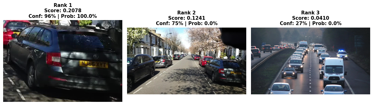
text_queries = [
"a grey skoda car parked on a residential street",
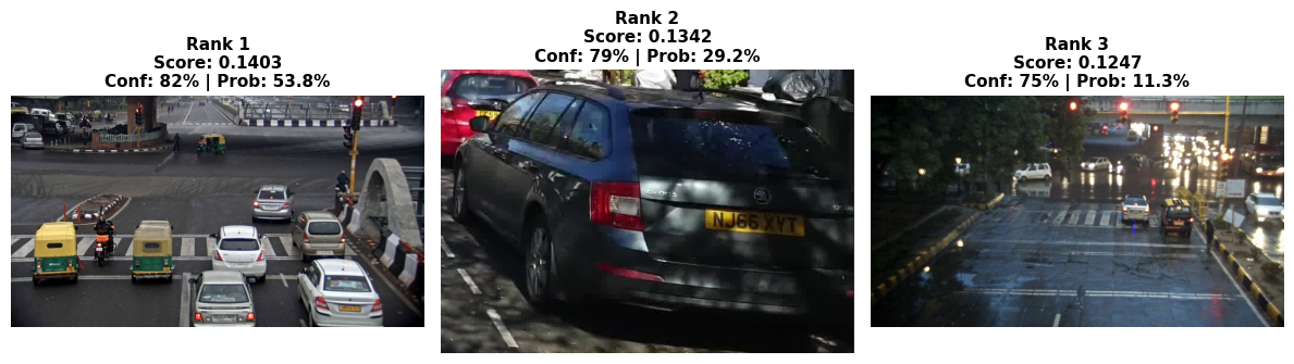
"vehicle lane splitting in traffic jam",
"orange mustang with yellow number plate",
"an ambulance in traffic with police car",
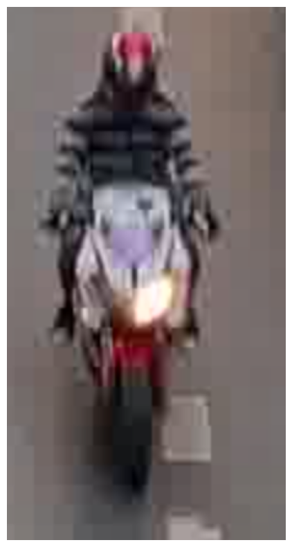
"a person in striped clothing on a motorcycle",
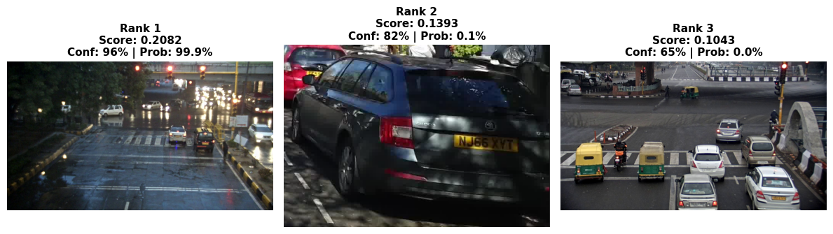
"a black van with yellow stripes on wet street and red light",
"a silver sedan car crossing intersection with traffic light",
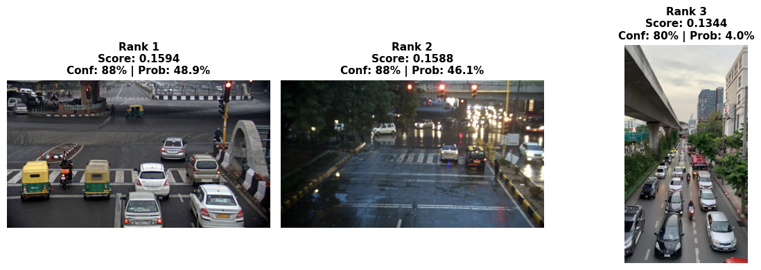
"traffic light on intersection",
]
test_text_to_image_retrieval(Path("../models/images/"), text_queries)
Found 11 images
Embedded 11 images → shape: torch.Size([11, 2048])

============================================================
Query: 'a grey skoda car parked on a residential street'
============================================================
============================================================
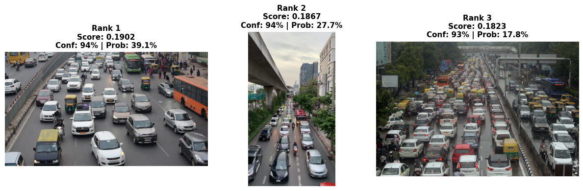
Query: 'vehicle lane splitting in traffic jam'
============================================================
============================================================
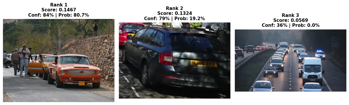
Query: 'orange mustang with yellow number plate'
============================================================
============================================================
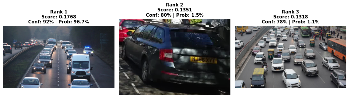
Query: 'an ambulance in traffic with police car'
============================================================
============================================================
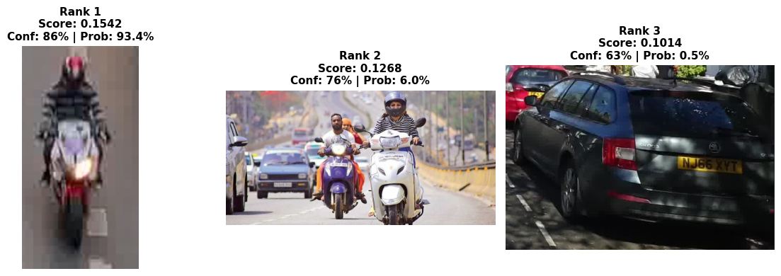
Query: 'a person in striped clothing on a motorcycle'
============================================================
============================================================
Query: 'a black van with yellow stripes on wet street and red light'
============================================================
============================================================
Query: 'a silver sedan car crossing intersection with traffic light'
============================================================
============================================================
Query: 'traffic light on intersection'
============================================================
Debugging text-image retrieval#
Undestand token sensitivity or impact on retrieval
The text encoder averages all token embeddings. More tokens = less weight per concept or attributes. Based on how Dinotxt was trained - the model works best when your queries match the distribution of captions it was trained on — which are typically short (Common crawl captions), simple descriptions of what’s visible.
Dominant and non-dominant
In a full scene or frame embedding, small objects like the “person in stripped clothing riding motorcyle” would barely make to the model’s attention (2% pixels)
Dominant: Traffic scene, multiple vehicles, road context (80%+ of image)
Non-dominant: Motorcyclist (maybe 5-10% of pixels)
Barely visible: Striped shirt, red helmet (< 2% of pixels)
def debug_dominant_objects_in_image(image_path, prompts):
    stripes_img = Image.open(image_path).convert("RGB")
    _, ax = plt.subplots(figsize=(8,8))
    ax.imshow(stripes_img)
    ax.axis('off')
    plt.tight_layout()
    plt.show()

    image_tensor = torch.stack([image_preprocess(stripes_img)]).cuda()

    with torch.autocast('cuda', dtype=torch.float):
        with torch.no_grad():
            image_features = model.encode_image(image_tensor)
            image_features /= image_features.norm(dim=-1, keepdim=True)

    debug_tokens = tokenizer.tokenize(prompts).cuda()
    with torch.autocast('cuda', dtype=torch.float):
        with torch.no_grad():
            debug_text_features = model.encode_text(debug_tokens)
            debug_text_features /= debug_text_features.norm(dim=-1, keepdim=True)

    debug_similarities = (debug_text_features @ image_features.T).cpu().float().numpy().flatten()
    confidence = torch.sigmoid(torch.tensor((debug_similarities - threshold) * temperature)).numpy()

    sorted_indices = debug_similarities.argsort()[::-1]
    print("="*70)
    print(f"Independent Confidence (threshold={threshold}, temp={temperature})")
    print("="*70)
    print(f"{'Conf':>6} | {'Score':>6} | Query")
    print("-"*70)
    for idx in sorted_indices:
        score = debug_similarities[idx]
        conf = confidence[idx]
        print(f"{conf:>6.1%} | {score:>7.4f} | {prompts[idx]}")
prompts = [
    "a person on a red motorcycle",

    "a motorcyclist in traffic",

    "a person wearing a red helmet",
    "a person wearing a helmet on a motorcycle",
    "a person in striped clothing on a red motorcycle",

    "a photo of a motorcyclist wearing a red helmet",
    "a photo of a person in a striped shirt on a motorcycle",

    "person on motorcycle wearing striped shirt and red helmet",
]

debug_dominant_objects_in_image("../models/images/stripes.jpg", prompts)
debug_dominant_objects_in_image("../models/images/stripes_crop.png", prompts)
======================================================================
Independent Confidence (threshold=0.08, temp=25.0)
======================================================================
  Conf |  Score | Query
----------------------------------------------------------------------
 87.4% |  0.1576 | a motorcyclist in traffic
 53.0% |  0.0849 | a person on a red motorcycle
 50.2% |  0.0804 | a photo of a motorcyclist wearing a red helmet
 47.9% |  0.0766 | a person wearing a helmet on a motorcycle
 39.6% |  0.0630 | a person in striped clothing on a red motorcycle
 38.9% |  0.0619 | person on motorcycle wearing striped shirt and red helmet
 37.0% |  0.0587 | a photo of a person in a striped shirt on a motorcycle
 31.4% |  0.0487 | a person wearing a red helmet
======================================================================
Independent Confidence (threshold=0.08, temp=25.0)
======================================================================
  Conf |  Score | Query
----------------------------------------------------------------------
 87.2% |  0.1567 | a motorcyclist in traffic
 84.2% |  0.1468 | a person in striped clothing on a red motorcycle
 81.4% |  0.1391 | a person on a red motorcycle
 81.1% |  0.1382 | a photo of a person in a striped shirt on a motorcycle
 79.2% |  0.1336 | person on motorcycle wearing striped shirt and red helmet
 77.2% |  0.1287 | a person wearing a helmet on a motorcycle
 76.4% |  0.1271 | a photo of a motorcyclist wearing a red helmet
 46.7% |  0.0748 | a person wearing a red helmet
Generic attribtues over specific attributes e.g. stripped clothing VS stripped shirt or tshirt. Context beats attributes e.g. a motorcyclist in traffic (87%) a person wearing a red helmet (46%)
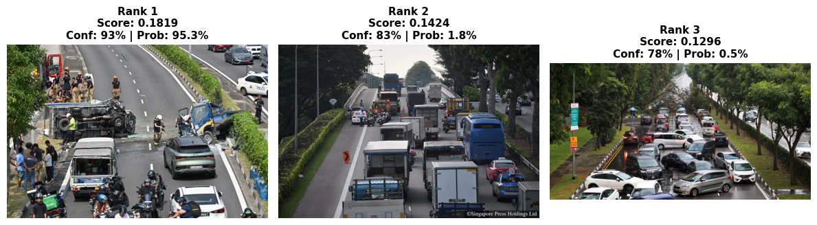
text_queries = [
"accident on the road",
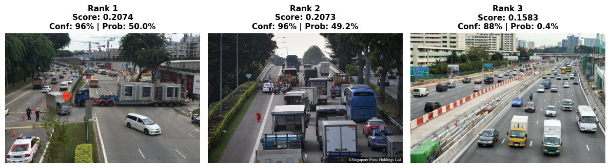
"large trailer breaking down while transporting concrete slabs along Upper Serangoon Road",
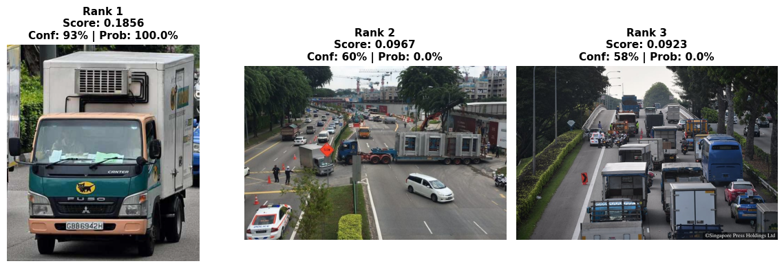
"green fuso truck with black cat sticker",
"yamato transport truck"
]
test_text_to_image_retrieval(Path("../models/sg_dataset/"), text_queries)
Found 20 images
Embedded 20 images → shape: torch.Size([20, 2048])

============================================================
Query: 'accident on the road'
============================================================
============================================================
Query: 'large trailer breaking down while transporting concrete slabs along Upper Serangoon Road'
============================================================
============================================================
Query: 'green fuso truck with black cat sticker'
============================================================
============================================================
Query: 'yamato transport truck'
============================================================
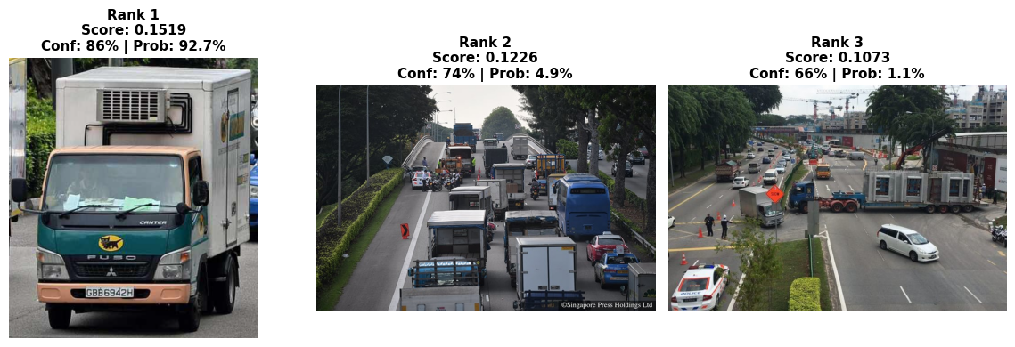
https://www.torque.com.sg/news/traffic-chaos-trailer-breaks/