◉ What the heck is Bigrams#
A bigram or digram is a sequence of two adjacent elements from a string of tokens, which are typically letters, syllables, or words.
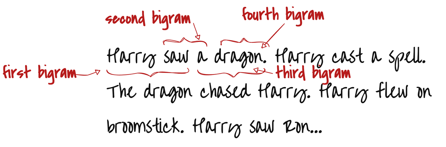
Example: From the sentence: “Harry flew on broomstick.” We can find these bigrams:
Harry flew
flew on
on broomstick
broomstick .
Each pair is a bigram — two words that are side-by-side.
A bigram language statistical model is a language model that predicts the likelihood of a word given its preceding word. In other words, it models the probability of a word occurring based on the word that precedes it.
We can see that our text has 4 relevant bigrams that start with ‘Harry’. Two of them lead to the word ‘saw’, while other leads to either ‘cast’ or ‘flew’. This means that ‘Harry saw something’ is twice as likely as ‘Harry cast’ or ‘Harry flew’
If we start with “a” as the starting word, the model (based on the probability) might say:
→ a → dragon → chased → Harry
Remember seeing next-word suggestions while typing messages on your phone? That’s the bigram model at work!#

Building a character Bigrams from names dataset#
We will start with a dataset with 32K unique english names.
words = open('names.txt', 'r').read().splitlines()
print(f"first 10 names from dataset {words[:10]}")
print(f"Length of dataset {len(words)}")
print(f"Smallest name size {min(len(w) for w in words)}")
print(f"longest name size {max(len(w) for w in words)}")
first 10 names from dataset ['emma', 'olivia', 'ava', 'isabella', 'sophia', 'charlotte', 'mia', 'amelia', 'harper', 'evelyn']
Length of dataset 32033
Smallest name size 2
longest name size 15
How would we create character pairs from single name?
"""
name = 'John' and name[1:] = 'ohn'
zip(name, name[1:]) = [('J', 'o'), ('o', 'h'), ('h', 'n')]
the last 'n' from name would be discarded since there is no pair for it in name[1:]

This is useful to train bigram models, where we want to predict the next character given the current character.
"""

name = 'John'
for ch1, ch2 in zip(name, name[1:]):
    print(ch1, ch2)
J o
o h
h n
… and finally attach a character token to indicate start and end of the name along with a count to indicate the number of times the pair appeared in the text (single word).
# Function to build character bigram model with the start and end tokens
# count the number of times each bigram appears in the list of words
# e.g. possibility of 'n' after 'a' is 5438, whereas after 'e' is 2675 from the dataset
# ('a', 'n'), 5438)
# ('e', 'n'), 2675)
def create_char_bigram_model(words):
    bigram_model = {}
    for w in words:
        chs = ['<S>'] + list(w) + ['<E>']
        for ch1, ch2 in zip(chs, chs[1:]):
            bigram = (ch1, ch2)
            bigram_model[bigram] = bigram_model.get(bigram, 0) + 1
    return bigram_model

def sort(bigram_model):
    # sort the bigram model by frequency
    return sorted(bigram_model.items(), key = lambda kv: -kv[1])
name = 'John'
respone = create_char_bigram_model([name])
sort(respone)
[(('<S>', 'J'), 1),
 (('J', 'o'), 1),
 (('o', 'h'), 1),
 (('h', 'n'), 1),
 (('n', '<E>'), 1)]
Creating character bigrams from the names dataset and displaying the top 10 most common pairs of characters.
sort(create_char_bigram_model(words))[:10]
[(('n', '<E>'), 6763),
 (('a', '<E>'), 6640),
 (('a', 'n'), 5438),
 (('<S>', 'a'), 4410),
 (('e', '<E>'), 3983),
 (('a', 'r'), 3264),
 (('e', 'l'), 3248),
 (('r', 'i'), 3033),
 (('n', 'a'), 2977),
 (('<S>', 'k'), 2963)]
Lets do PyTorch instead#
As its easier to do manuplation on tensor than numpy array
import torch
A 27x27 tensor to represent the bigrams i.e. it will hold the count of each character pair where the i represents the first character and j represents the second character. Note that we are using . as the start and end token.
# 26 Charaacters in the alphabet + . (token to indicate start and end of word)
# create a tensor of 27x27 to store the bigram counts
N = torch.zeros((27, 27), dtype=torch.int32)
our characters would be indexed as integers from 1 to 27. We’ll reserve 0 to represent the padding token (start and end char).
chars = sorted(list(set(''.join(words))))
# s (str) to i (index)
stoi = {s:i+1 for i,s in enumerate(chars)}
stoi['.'] = 0
# rever the array
itos = {i:s for s,i in stoi.items()}

print(f"stoi['a'] = {stoi['a']}")
print(f"itos[1] = {itos[1]}")
stoi['a'] = 1
itos[1] = a
for w in words:
  chs = ['.'] + list(w) + ['.']
  for ch1, ch2 in zip(chs, chs[1:]):
    ix1 = stoi[ch1]
    ix2 = stoi[ch2]
    N[ix1, ix2] += 1

print(f"N[stoi['a'], stoi['n']] = count of 'a' and 'n' = {N[stoi['a'], stoi['n']]}")
N[stoi['a'], stoi['n']] = count of 'a' and 'n' = 5438
Character Bigrams model represented as 27x27 tensor#
import matplotlib.pyplot as plt
%matplotlib inline

plt.figure(figsize=(16,16))
plt.imshow(N, cmap='Blues')
for i in range(27):
    for j in range(27):
        chstr = itos[i] + itos[j]
        plt.text(j, i, chstr, ha="center", va="bottom", color='gray')
        plt.text(j, i, N[i, j].item(), ha="center", va="top", color='gray')
plt.axis('off');

# the 0th element never happened since the word cannot be empty
# the first row represents start character, and column represent the end character
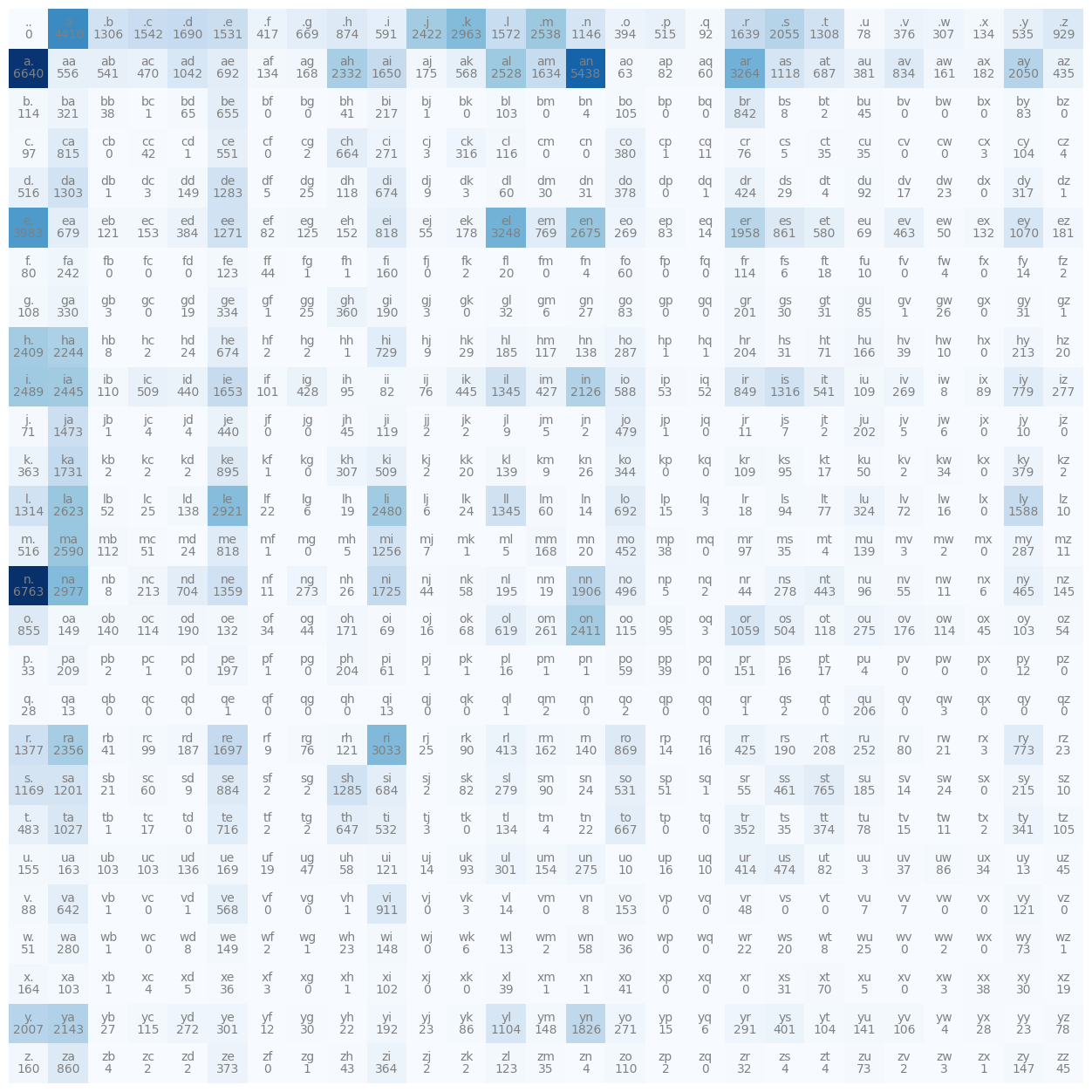
# start character counts
N[0] # equal to N[0, :]
tensor([   0, 4410, 1306, 1542, 1690, 1531,  417,  669,  874,  591, 2422, 2963,
        1572, 2538, 1146,  394,  515,   92, 1639, 2055, 1308,   78,  376,  307,
         134,  535,  929], dtype=torch.int32)
Probabibility distribution#
A probability distribution disributes the total probability (100%) accross all the possible outcomes such that the sum of all the probabilities is equal to 1.0 (100%). In our bigram model, the outcomes are the counts of each character pair.
💡Lets undestand the concept
Create a random tesnor of size 3
Normalize the tensor to get the probability distribution
Draw 15 samples using the probability distribution
Note the probability of first element (0) is 60% and the second element (1) is 30%… hence the count of 0 is higher than 1 in the samples drawn.
# create a deterministic random number generator
gen = torch.Generator().manual_seed(2147483647)
# create a random tensor of size 3
rand_tensor = torch.rand(3, generator=gen)
# normalize the random tensor to create a probability distribution
p_dist = rand_tensor / rand_tensor.sum()
print(f"rand_tensor = {rand_tensor}")
print(f"probability dist = {p_dist}")

print(torch.multinomial(p_dist, num_samples=15, replacement=True, generator=gen))
rand_tensor = tensor([0.7081, 0.3542, 0.1054])
probability dist = tensor([0.6064, 0.3033, 0.0903])
tensor([1, 1, 2, 0, 0, 2, 1, 1, 0, 0, 0, 1, 1, 0, 0])
We apply the same concept to our char bigram tensor. We’ll use the first row of our tensor to plot the probability distribution, and then sample a character based on that distribution.
p = N[0].float()
p = p / p.sum()
p
tensor([0.0000, 0.1377, 0.0408, 0.0481, 0.0528, 0.0478, 0.0130, 0.0209, 0.0273,
        0.0184, 0.0756, 0.0925, 0.0491, 0.0792, 0.0358, 0.0123, 0.0161, 0.0029,
        0.0512, 0.0642, 0.0408, 0.0024, 0.0117, 0.0096, 0.0042, 0.0167, 0.0290])
# deterministic sampling
g = torch.Generator().manual_seed(2147483647)

samples = torch.multinomial(p, num_samples=3, replacement=True, generator=g)
print(f"ix = {samples}")
for i in samples:
    print(f"itos[{i.item()}] = {itos[i.item()]}")
ix = tensor([13, 19, 14])
itos[13] = m
itos[19] = s
itos[14] = n
Creating a probability distribution Tensor#
Understanding the Bigram Tensor in PyTorch
The bigram tensor N is a 27x27 tensor, where:
Each row represents the first character of a bigram indexed with
i.Each column represents the second character indexed with
j.The value at position (i, j) in the tensor indicates the number of times the bigram formed by the i-th and j-th characters appears in the names dataset.
Determining the Most Likely Next Character
To find the most likely next character after a given character i, we:
Look at the i-th row of the tensor.
Identify the column
jwith the highest value — this represents the character that most frequently follows characteri.
Example:
If the first character is 'a', we check the second row (index 1).
If the highest value in that row is at column 'n', with a count of 5438, then 'n' is the most likely character to follow 'a'.
Creating a Probability Distribution Tensor
To convert the count-based tensor into a probability distribution, we:
Divide each element in a row by the sum of that row.
This ensures that each row becomes a valid probability distribution, where the values sum to 1.
Using PyTorch Broadcasting
We can achieve this efficiently using PyTorch broadcasting:
# N is the 27x27 count tensor
P = N.float()
prob_dist = P / P.sum(1, keepdim=True)
P.sum(1, keepdim=True)computes a 27x1 tensor containing the sum of each row creating a column tensor of shape 27x1.PyTorch automatically broadcasts this tensor across the 27 columns when performing the division.
The result is a 27x27 tensor of probabilities.
Learn more about PyTorch broadcasting here: 🔗 https://pytorch.org/docs/stable/notes/broadcasting.html
P = N.float()
# P = P / P.sum(1, keepdim=True)  # Creates new tensor and not memory efficient
P /= P.sum(1, keepdim=True) # creates in-place and is memory efficient
P[0, :].sum() # should normalise to 1
print(f'Probability distribution of first row \n{P[1, :]}')
print(f'And it sum up to = {P[1, :].sum()}')
Probability distribution of first row
tensor([0.1960, 0.0164, 0.0160, 0.0139, 0.0308, 0.0204, 0.0040, 0.0050, 0.0688,
        0.0487, 0.0052, 0.0168, 0.0746, 0.0482, 0.1605, 0.0019, 0.0024, 0.0018,
        0.0963, 0.0330, 0.0203, 0.0112, 0.0246, 0.0048, 0.0054, 0.0605, 0.0128])
And it sum up to = 1.0
Sampling#
Given our probability distribution, we can sample the next character based on the likelihood of each character following the previous one. This allows us to generate new names, character by character.
Even if some of the generated names looks “rubbish,” the model is still quite respectable — especially considering it’s only using 2 characters at a time (a bigram) to make predictions…
g = torch.Generator().manual_seed(2147483647)

for i in range(10):
    out = []
    ix = 0
    while True:
        p = P[ix]
        ix = torch.multinomial(p, num_samples=1, replacement=True, generator=g).item()
        out.append(itos[ix])
        if ix == 0:
            break

    print(''.join(out))
cexze.
momasurailezitynn.
konimittain.
llayn.
ka.
da.
staiyaubrtthrigotai.
moliellavo.
ke.
teda.
Measure the quality of the model#
Maximum Likelihood Estimation (MLE) 🔗 Wikipedia: Maximum Likelihood Estimation
Maximum Likelihood Estimation (MLE) is a method used to estimate the parameters of a statistical model. Given a set of observations, MLE finds the parameter values that maximize the likelihood of observing the given data under the model.
How MLE Works in Our Case
In our bigram model:
The
Ntensor represents the observations, i.e., the counts of each bigram (how often each character pair appears).The
Ptensor contains the probabilities (our model’s parameters), calculated by normalizingNso each row sums to 1.
According to MLE, the likelihood of the data is the product of the probabilities of each observation given the model parameters. So, during training, we want to maximize this product — in other words, increase the likelihood of the observed bigram counts under the current probability distribution.
The Problem: Tiny Probabilities
When working with probabilities, we often deal with very small numbers. Multiplying many small probabilities together can lead to extremely small results, which computers can struggle to represent. This is called numerical underflow.
Example:
If you multiply 0.0001 by itself 100 times:
0.0001^100 = 1e-400
This number is so small it may not be stored accurately in memory, especially with standard floating-point precision.
Log-Likelihood
To avoid this issue, we use logarithms (ring some bells from your high school days???). The log of a product is equal to the sum of the logs:
This transformation makes the math numerically stable and easier to handle. Also note that the logarithm is a monotonic function, meaning it preserves the order of numbers. So, if p1 > p2, then log(p1) > log(p2).
So… Our GOAL is to maximize the likelihood of the data with respect to the model parameters (statistical modeling).
This is equivalent to:
Maximizing the log-likelihood (because log is a monotonic function, it preserves order)
Minimizing the negative log-likelihood (common in loss functions for training models)
Minimizing the average negative log-likelihood (which gives us a per-sample loss, useful for gradient-based optimization)
Compute the log likelihood and Negative log likelihood on first 3 words
log_likelihood = 0.0
n = 0

for w in words[:3]:
  chs = ['.'] + list(w) + ['.']
  for ch1, ch2 in zip(chs, chs[1:]):
    ix1 = stoi[ch1]
    ix2 = stoi[ch2]
    prob = P[ix1, ix2]
    logprob = torch.log(prob)
    log_likelihood += logprob
    n += 1
    print(f'{ch1}{ch2}: {prob:.4f} {logprob:.4f}')

print(f'{log_likelihood=}')
nll = -log_likelihood
print(f'{nll=}')
print(f'Loss: {nll/n}')
.e: 0.0478 -3.0408
em: 0.0377 -3.2793
mm: 0.0253 -3.6772
ma: 0.3899 -0.9418
a.: 0.1960 -1.6299
.o: 0.0123 -4.3982
ol: 0.0780 -2.5508
li: 0.1777 -1.7278
iv: 0.0152 -4.1867
vi: 0.3541 -1.0383
ia: 0.1381 -1.9796
a.: 0.1960 -1.6299
.a: 0.1377 -1.9829
av: 0.0246 -3.7045
va: 0.2495 -1.3882
a.: 0.1960 -1.6299
log_likelihood=tensor(-38.7856)
nll=tensor(38.7856)
Loss: 2.424102306365967
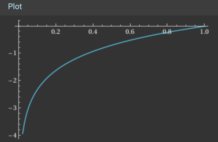
Log(x) for x 0 to 1: you notice that log(1) is zero, and as it changes to less than 1, when x goes negative all the way to -inf
this is why we took the negative log likelihood. The average for NLL is basically used for simplifying the loss function.
So…#
tried training a bigram model that predicts the next character based on the previous character.
created a tensor
Nrepresenting the counts of bigrams, computed manually from a dataset of 32,000 names.from these counts, we have a tensor
Prepresenting the probabilities of each bigram by normalizingN.using these probabilities, we can sample new words from the model — generating character sequences one step at a time.
and… use a loss function based on Negative Log-Likelihood (NLL) to evaluate the model.
The lower the NLL, the better the model fits the observed data.
Alternate appraoch using Neural Networks#
We will start by creating a training set of the bigrams. Example: in the name emma, there are 5 bigrams:
. e
e m
m m
m a
a .
So when we input e, we expect our neural network to output m.
# create the training set of bigrams (x,y)
# xs is the input character and ys is the target output
xs, ys = [], []

for w in words[:1]:
  chs = ['.'] + list(w) + ['.']
  for ch1, ch2 in zip(chs, chs[1:]):
    ix1 = stoi[ch1]
    ix2 = stoi[ch2]
    print(ch1, ch2)
    xs.append(ix1)
    ys.append(ix2)

xs = torch.tensor(xs)
ys = torch.tensor(ys)
print(f'xs: {xs}')
print(f'ys: {ys}')
. e
e m
m m
m a
a .
xs: tensor([ 0,  5, 13, 13,  1])
ys: tensor([ 5, 13, 13,  1,  0])
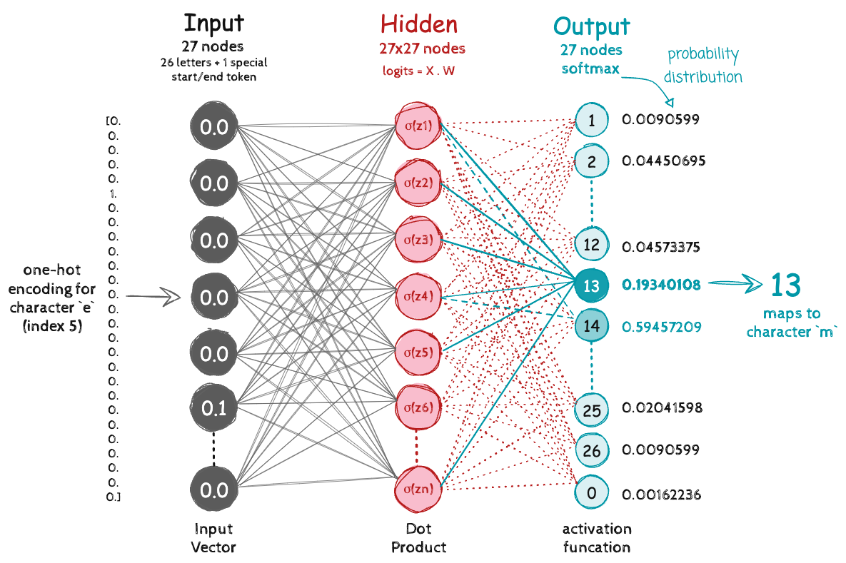
In a character bigram neural network, both the input and output layers are shaped as 27×1 tensors, representing the 27 possible characters (26 letters + 1 special start/end token).
Our training data tensor xs is made up of integers, where:
0represents the start/end character,5represents the character ‘e’,13represents ‘m’, and so on.
To feed these into the network, we would need to convert each integers into tensors. We could use one-hot encoding, a common method for representing categorical data numerically.
In one-hot encoding, each character can be represented by a vector of shape 27 where:
The index corresponding to the character is set to 1.
All other indices are set to 0.
Example:
If the character is 'm' (index 13), its one-hot encoding would be:
[0, 0, 0, ..., 0, 1, 0, ..., 0] ← (1 at position 13)
import torch.nn.functional as F
xenc = F.one_hot(xs, num_classes=27).float()
xenc
tensor([[1., 0., 0., 0., 0., 0., 0., 0., 0., 0., 0., 0., 0., 0., 0., 0., 0., 0.,
         0., 0., 0., 0., 0., 0., 0., 0., 0.],
        [0., 0., 0., 0., 0., 1., 0., 0., 0., 0., 0., 0., 0., 0., 0., 0., 0., 0.,
         0., 0., 0., 0., 0., 0., 0., 0., 0.],
        [0., 0., 0., 0., 0., 0., 0., 0., 0., 0., 0., 0., 0., 1., 0., 0., 0., 0.,
         0., 0., 0., 0., 0., 0., 0., 0., 0.],
        [0., 0., 0., 0., 0., 0., 0., 0., 0., 0., 0., 0., 0., 1., 0., 0., 0., 0.,
         0., 0., 0., 0., 0., 0., 0., 0., 0.],
        [0., 1., 0., 0., 0., 0., 0., 0., 0., 0., 0., 0., 0., 0., 0., 0., 0., 0.,
         0., 0., 0., 0., 0., 0., 0., 0., 0.]])
xenc.shape
torch.Size([5, 27])
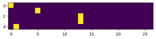
# respective one-hot encoding bit is turned on in the figure
plt.imshow(xenc)
<matplotlib.image.AxesImage at 0x11fc716f0>
xenc.dtype
torch.float32
Forward Pass in a Character Bigram Neural Network#
We create a random weight matrix using a standard normal distribution, similar to how we initialized our N tensor in the count-based approach:
W = torch.randn((27, 27))
Let’s multiply a batch (size 5 for emma) of one-hot encoded vectors xenc with the weight matrix W:
PyTorch will automatically handle the matrix multiplication for us, and we can use the @ operator to perform the dot product.
logits = xenc @ W  # Matrix multiplication
# shape: [batch_size, 27] @ [27, 27] => [batch_size, 27]
logits
tensor([[-0.3419,  0.0760, -1.4656, -2.1475, -1.2871,  0.5640,  0.7037,  0.0488,
         -0.8625,  0.4855,  0.9117,  0.7930,  0.3225, -0.6081,  0.3359,  1.1189,
         -0.3551, -1.9349,  0.1892,  0.1096,  0.5020, -1.4333,  0.6469, -0.2417,
         -0.1678, -0.2421, -0.1138],
        [-0.8451,  1.4149,  0.9330, -0.9055, -0.0837, -0.5023, -0.5673, -0.2823,
          1.0445,  1.5295,  0.2718,  1.5050,  1.2082, -0.4183,  1.4257,  1.4903,
          0.5934, -0.1868, -1.6786, -0.2488, -0.1913,  1.0501, -0.3789, -1.2747,
          0.7680, -0.4310, -0.5766],
        [-0.4051, -0.0528,  1.0928,  0.0425, -1.8870,  0.3698, -0.9891,  0.5949,
          1.2641, -1.1659,  0.5657,  1.4391, -0.6306, -1.5472, -0.0258,  0.0122,
         -0.4690,  0.1881, -1.0994,  0.6661,  0.6150,  0.9037, -2.3169,  2.5160,
          0.4834,  0.3516, -0.6384],
        [-0.4051, -0.0528,  1.0928,  0.0425, -1.8870,  0.3698, -0.9891,  0.5949,
          1.2641, -1.1659,  0.5657,  1.4391, -0.6306, -1.5472, -0.0258,  0.0122,
         -0.4690,  0.1881, -1.0994,  0.6661,  0.6150,  0.9037, -2.3169,  2.5160,
          0.4834,  0.3516, -0.6384],
        [-1.2472,  0.9954, -1.4838, -0.9758, -0.3820,  0.3855, -0.3514, -0.1562,
          0.5565,  0.2106, -0.3916, -0.3628,  0.1993,  2.0544, -0.7253, -0.5915,
         -0.3486,  0.7160, -0.9597,  0.4873,  0.1986,  1.4308,  1.8924,  0.6137,
         -0.1563,  0.4788,  2.2193]])
⚠️ Challenge: Logits May Be Negative The challenge with the above dot product is that the output contains both positive and negative values. We need to move towards positive values in order to get the probability distribution. To convert them into non-negative values, we apply the exponential function:
counts = logits.exp() # Turns log-counts into positive values
Negative logits become small positive numbers (less than 1).
Positive logits become large positive numbers.
logits = xenc @ W # log-counts
counts = logits.exp() # equivalent N
probs = counts / counts.sum(1, keepdims=True)

print (f'xenc = {xenc[1]}')
print (f'logits = {logits[1]}')
print (f'Counts = {counts[1]}')
print (f'Probabilities = {probs[1]}')
probs[1].sum()
xenc = tensor([0., 0., 0., 0., 0., 1., 0., 0., 0., 0., 0., 0., 0., 0., 0., 0., 0., 0.,
        0., 0., 0., 0., 0., 0., 0., 0., 0.])
logits = tensor([-0.8451,  1.4149,  0.9330, -0.9055, -0.0837, -0.5023, -0.5673, -0.2823,
         1.0445,  1.5295,  0.2718,  1.5050,  1.2082, -0.4183,  1.4257,  1.4903,
         0.5934, -0.1868, -1.6786, -0.2488, -0.1913,  1.0501, -0.3789, -1.2747,
         0.7680, -0.4310, -0.5766])
Counts = tensor([0.4295, 4.1159, 2.5422, 0.4043, 0.9197, 0.6051, 0.5671, 0.7541, 2.8420,
        4.6160, 1.3123, 4.5042, 3.3474, 0.6582, 4.1608, 4.4386, 1.8102, 0.8296,
        0.1866, 0.7797, 0.8259, 2.8580, 0.6846, 0.2795, 2.1555, 0.6499, 0.5618])
Probabilities = tensor([0.0090, 0.0860, 0.0531, 0.0085, 0.0192, 0.0126, 0.0119, 0.0158, 0.0594,
        0.0965, 0.0274, 0.0942, 0.0700, 0.0138, 0.0870, 0.0928, 0.0378, 0.0173,
        0.0039, 0.0163, 0.0173, 0.0597, 0.0143, 0.0058, 0.0451, 0.0136, 0.0117])
tensor(1.)
At the moment, the probabilities are quite rubbish given we started with random weights with standard normal distribution. Our next goal is to train the model to learn the weights that would give us a good probability distribution.
# Input data with first character from word `emma` (5 possible samples from bigram)
xs
tensor([ 0, 5, 13, 13, 1])
# similar next character from word `emma` (5 possible samples from bigram) - labels
ys
tensor([ 5, 13, 13, 1, 0])
# randomly initialize 27 neurons' weights. each neuron receives 27 inputs
g = torch.Generator().manual_seed(2147483647)
# g = torch.Generator().manual_seed(2147483647 + 1)
W = torch.randn((27, 27), generator=g)
And finally normalize the counts by dividing each row by its sum to get probabilities: i.e. Convert to Probability Distribution (Softmax)
Softmax : Exponent the logits and divide by the sum of all exponentials of logits to create a probability distribution
xenc = F.one_hot(xs, num_classes=27).float() # input to the network: one-hot encoding
logits = xenc @ W # predict log-counts

# Softmax Activation
counts = logits.exp() # counts, equivalent to N
probs = counts / counts.sum(1, keepdims=True) # probabilities for next character
probs.shape
torch.Size([5, 27])
def get_model_confidence(nlls):
    avg_nll = nlls.mean().item()
    loss = torch.tensor(avg_nll)
    avg_prob = torch.exp(-loss)
    return (avg_prob * 100).item()
# 5 input from the word `emma`
print('Running the network for the word emma which consist 5 inputs (first character) and 5 outputs (next character)')
nlls = torch.zeros(5)
for i in range(5):
  # i-th bigram:
  x = xs[i].item() # input character index
  y = ys[i].item() # label character index
  print('--------')
  print(f'bigram example {i+1}: {itos[x]}{itos[y]} (indexes {x},{y})')
  print('input to the neural net:', x)
  print('output probabilities from the neural net:', probs[i])
  print('label (actual next character):', y)
  p = probs[i, y]
  print('probability assigned by the net to the the correct character:', p.item())
  logp = torch.log(p)
  print('log likelihood:', logp.item())
  nll = -logp
  print('negative log likelihood:', nll.item())
  nlls[i] = nll

print('=========')

print('average negative log likelihood, i.e. loss =', nlls.mean().item())
print(f"models confidence: {get_model_confidence(nlls):.2f}%")
Running the network for the word emma which consist 5 inputs (first character) and 5 outputs (next character)
--------
bigram example 1: .e (indexes 0,5)
input to the neural net: 0
output probabilities from the neural net: tensor([0.0607, 0.0100, 0.0123, 0.0042, 0.0168, 0.0123, 0.0027, 0.0232, 0.0137,
        0.0313, 0.0079, 0.0278, 0.0091, 0.0082, 0.0500, 0.2378, 0.0603, 0.0025,
        0.0249, 0.0055, 0.0339, 0.0109, 0.0029, 0.0198, 0.0118, 0.1537, 0.1459])
label (actual next character): 5
probability assigned by the net to the the correct character: 0.012286253273487091
log likelihood: -4.3992743492126465
negative log likelihood: 4.3992743492126465
--------
bigram example 2: em (indexes 5,13)
input to the neural net: 5
output probabilities from the neural net: tensor([0.0290, 0.0796, 0.0248, 0.0521, 0.1989, 0.0289, 0.0094, 0.0335, 0.0097,
        0.0301, 0.0702, 0.0228, 0.0115, 0.0181, 0.0108, 0.0315, 0.0291, 0.0045,
        0.0916, 0.0215, 0.0486, 0.0300, 0.0501, 0.0027, 0.0118, 0.0022, 0.0472])
label (actual next character): 13
probability assigned by the net to the the correct character: 0.018050702288746834
log likelihood: -4.014570713043213
negative log likelihood: 4.014570713043213
--------
bigram example 3: mm (indexes 13,13)
input to the neural net: 13
output probabilities from the neural net: tensor([0.0312, 0.0737, 0.0484, 0.0333, 0.0674, 0.0200, 0.0263, 0.0249, 0.1226,
        0.0164, 0.0075, 0.0789, 0.0131, 0.0267, 0.0147, 0.0112, 0.0585, 0.0121,
        0.0650, 0.0058, 0.0208, 0.0078, 0.0133, 0.0203, 0.1204, 0.0469, 0.0126])
label (actual next character): 13
probability assigned by the net to the the correct character: 0.026691533625125885
log likelihood: -3.623408794403076
negative log likelihood: 3.623408794403076
--------
bigram example 4: ma (indexes 13,1)
input to the neural net: 13
output probabilities from the neural net: tensor([0.0312, 0.0737, 0.0484, 0.0333, 0.0674, 0.0200, 0.0263, 0.0249, 0.1226,
        0.0164, 0.0075, 0.0789, 0.0131, 0.0267, 0.0147, 0.0112, 0.0585, 0.0121,
        0.0650, 0.0058, 0.0208, 0.0078, 0.0133, 0.0203, 0.1204, 0.0469, 0.0126])
label (actual next character): 1
probability assigned by the net to the the correct character: 0.07367684692144394
log likelihood: -2.6080667972564697
negative log likelihood: 2.6080667972564697
--------
bigram example 5: a. (indexes 1,0)
input to the neural net: 1
output probabilities from the neural net: tensor([0.0150, 0.0086, 0.0396, 0.0100, 0.0606, 0.0308, 0.1084, 0.0131, 0.0125,
        0.0048, 0.1024, 0.0086, 0.0988, 0.0112, 0.0232, 0.0207, 0.0408, 0.0078,
        0.0899, 0.0531, 0.0463, 0.0309, 0.0051, 0.0329, 0.0654, 0.0503, 0.0091])
label (actual next character): 0
probability assigned by the net to the the correct character: 0.0149775305762887
log likelihood: -4.201204299926758
negative log likelihood: 4.201204299926758
=========
average negative log likelihood, i.e. loss = 3.7693049907684326
models confidence: 2.31%
The confidence of the model is very low and its understood as we started with random weights. We can simulate by manually adding +1 to the SEED i.e. torch.Generator().manual_seed(2147483647 + 1) and see the loss changing (improve or worsen) - but that’s amatuer approach to improving parameters and not how we would want to update the weights. We will find the optimization through backpropogation and gradient descent.
Lets do the drill again…
# Input data with first character from word `emma` (5 possible samples from bigram)
xs
tensor([ 0, 5, 13, 13, 1])
# similar next character from word `emma` (5 possible samples from bigram) - labels
ys
tensor([ 5, 13, 13, 1, 0])
Model optimization using Backpropagation (Gradient Descent)#
All of the steps in Forward Pass can be considered as layers or differential operation that can be backpropogated. This means we can use backpropagation to train the model by minimizing the loss i.e. updating the weights.
Notice how we set requires_grad=True when creating the weights tensor.
This tells PyTorch to track operations on the tensor so it can compute gradients during backpropagation.
When we later call loss.backward(), PyTorch automatically calculates the gradient of the loss with respect to the weights.
These gradients are then used to update the weights using an optimization algorithm, such as Stochastic Gradient Descent (SGD).
g = torch.Generator().manual_seed(2147483647)
W = torch.randn((27, 27), generator=g, requires_grad=True)
# forward pass
xenc = F.one_hot(xs, num_classes=27).float() # input to the network: one-hot encoding
logits = xenc @ W # predict log-counts
counts = logits.exp() # counts, equivalent to N
probs = counts / counts.sum(1, keepdims=True) # probabilities for next character
specifically for our input emma, we are interested in below probabilities in order to improve them with respect to the output labels ys…
probs[0, 5], probs[1, 13], probs[2, 13], probs[3, 1], probs[4, 0]
(tensor(0.0123, grad_fn=<SelectBackward0>),
 tensor(0.0181, grad_fn=<SelectBackward0>),
 tensor(0.0267, grad_fn=<SelectBackward0>),
 tensor(0.0737, grad_fn=<SelectBackward0>),
 tensor(0.0150, grad_fn=<SelectBackward0>))
# Better way to access them instead of hardcoding the index
print(torch.arange(5))
probs[torch.arange(5), ys]
tensor([0, 1, 2, 3, 4])
tensor([0.0123, 0.0181, 0.0267, 0.0737, 0.0150], grad_fn=<IndexBackward0>)
now we can easily compute the loss by taking the negative log of the probabilities.
loss = -probs[torch.arange(5), ys].log().mean()
print(f"loss = {loss.item()}")
print(f'models confidence = {get_model_confidence(loss):.2f}%')
loss = 3.7693049907684326
models confidence = 2.31%
Backward Pass
# backward pass
print(W.grad)
W.grad = None # set to zero the gradient
loss.backward()
print(W.grad) # Notice that the gradient of the weights tensor is not zero after the backward pass
None
tensor([[ 0.0121,  0.0020,  0.0025,  0.0008,  0.0034, -0.1975,  0.0005,  0.0046,
          0.0027,  0.0063,  0.0016,  0.0056,  0.0018,  0.0016,  0.0100,  0.0476,
          0.0121,  0.0005,  0.0050,  0.0011,  0.0068,  0.0022,  0.0006,  0.0040,
          0.0024,  0.0307,  0.0292],
        [-0.1970,  0.0017,  0.0079,  0.0020,  0.0121,  0.0062,  0.0217,  0.0026,
          0.0025,  0.0010,  0.0205,  0.0017,  0.0198,  0.0022,  0.0046,  0.0041,
          0.0082,  0.0016,  0.0180,  0.0106,  0.0093,  0.0062,  0.0010,  0.0066,
          0.0131,  0.0101,  0.0018],
        [ 0.0000,  0.0000,  0.0000,  0.0000,  0.0000,  0.0000,  0.0000,  0.0000,
          0.0000,  0.0000,  0.0000,  0.0000,  0.0000,  0.0000,  0.0000,  0.0000,
          0.0000,  0.0000,  0.0000,  0.0000,  0.0000,  0.0000,  0.0000,  0.0000,
          0.0000,  0.0000,  0.0000],
        [ 0.0000,  0.0000,  0.0000,  0.0000,  0.0000,  0.0000,  0.0000,  0.0000,
          0.0000,  0.0000,  0.0000,  0.0000,  0.0000,  0.0000,  0.0000,  0.0000,
          0.0000,  0.0000,  0.0000,  0.0000,  0.0000,  0.0000,  0.0000,  0.0000,
          0.0000,  0.0000,  0.0000],
        [ 0.0000,  0.0000,  0.0000,  0.0000,  0.0000,  0.0000,  0.0000,  0.0000,
          0.0000,  0.0000,  0.0000,  0.0000,  0.0000,  0.0000,  0.0000,  0.0000,
          0.0000,  0.0000,  0.0000,  0.0000,  0.0000,  0.0000,  0.0000,  0.0000,
          0.0000,  0.0000,  0.0000],
        [ 0.0058,  0.0159,  0.0050,  0.0104,  0.0398,  0.0058,  0.0019,  0.0067,
          0.0019,  0.0060,  0.0140,  0.0046,  0.0023, -0.1964,  0.0022,  0.0063,
          0.0058,  0.0009,  0.0183,  0.0043,  0.0097,  0.0060,  0.0100,  0.0005,
          0.0024,  0.0004,  0.0094],
        [ 0.0000,  0.0000,  0.0000,  0.0000,  0.0000,  0.0000,  0.0000,  0.0000,
          0.0000,  0.0000,  0.0000,  0.0000,  0.0000,  0.0000,  0.0000,  0.0000,
          0.0000,  0.0000,  0.0000,  0.0000,  0.0000,  0.0000,  0.0000,  0.0000,
          0.0000,  0.0000,  0.0000],
        [ 0.0000,  0.0000,  0.0000,  0.0000,  0.0000,  0.0000,  0.0000,  0.0000,
          0.0000,  0.0000,  0.0000,  0.0000,  0.0000,  0.0000,  0.0000,  0.0000,
          0.0000,  0.0000,  0.0000,  0.0000,  0.0000,  0.0000,  0.0000,  0.0000,
          0.0000,  0.0000,  0.0000],
        [ 0.0000,  0.0000,  0.0000,  0.0000,  0.0000,  0.0000,  0.0000,  0.0000,
          0.0000,  0.0000,  0.0000,  0.0000,  0.0000,  0.0000,  0.0000,  0.0000,
          0.0000,  0.0000,  0.0000,  0.0000,  0.0000,  0.0000,  0.0000,  0.0000,
          0.0000,  0.0000,  0.0000],
        [ 0.0000,  0.0000,  0.0000,  0.0000,  0.0000,  0.0000,  0.0000,  0.0000,
          0.0000,  0.0000,  0.0000,  0.0000,  0.0000,  0.0000,  0.0000,  0.0000,
          0.0000,  0.0000,  0.0000,  0.0000,  0.0000,  0.0000,  0.0000,  0.0000,
          0.0000,  0.0000,  0.0000],
        [ 0.0000,  0.0000,  0.0000,  0.0000,  0.0000,  0.0000,  0.0000,  0.0000,
          0.0000,  0.0000,  0.0000,  0.0000,  0.0000,  0.0000,  0.0000,  0.0000,
          0.0000,  0.0000,  0.0000,  0.0000,  0.0000,  0.0000,  0.0000,  0.0000,
          0.0000,  0.0000,  0.0000],
        [ 0.0000,  0.0000,  0.0000,  0.0000,  0.0000,  0.0000,  0.0000,  0.0000,
          0.0000,  0.0000,  0.0000,  0.0000,  0.0000,  0.0000,  0.0000,  0.0000,
          0.0000,  0.0000,  0.0000,  0.0000,  0.0000,  0.0000,  0.0000,  0.0000,
          0.0000,  0.0000,  0.0000],
        [ 0.0000,  0.0000,  0.0000,  0.0000,  0.0000,  0.0000,  0.0000,  0.0000,
          0.0000,  0.0000,  0.0000,  0.0000,  0.0000,  0.0000,  0.0000,  0.0000,
          0.0000,  0.0000,  0.0000,  0.0000,  0.0000,  0.0000,  0.0000,  0.0000,
          0.0000,  0.0000,  0.0000],
        [ 0.0125, -0.1705,  0.0194,  0.0133,  0.0270,  0.0080,  0.0105,  0.0100,
          0.0490,  0.0066,  0.0030,  0.0316,  0.0052, -0.1893,  0.0059,  0.0045,
          0.0234,  0.0049,  0.0260,  0.0023,  0.0083,  0.0031,  0.0053,  0.0081,
          0.0482,  0.0187,  0.0051],
        [ 0.0000,  0.0000,  0.0000,  0.0000,  0.0000,  0.0000,  0.0000,  0.0000,
          0.0000,  0.0000,  0.0000,  0.0000,  0.0000,  0.0000,  0.0000,  0.0000,
          0.0000,  0.0000,  0.0000,  0.0000,  0.0000,  0.0000,  0.0000,  0.0000,
          0.0000,  0.0000,  0.0000],
        [ 0.0000,  0.0000,  0.0000,  0.0000,  0.0000,  0.0000,  0.0000,  0.0000,
          0.0000,  0.0000,  0.0000,  0.0000,  0.0000,  0.0000,  0.0000,  0.0000,
          0.0000,  0.0000,  0.0000,  0.0000,  0.0000,  0.0000,  0.0000,  0.0000,
          0.0000,  0.0000,  0.0000],
        [ 0.0000,  0.0000,  0.0000,  0.0000,  0.0000,  0.0000,  0.0000,  0.0000,
          0.0000,  0.0000,  0.0000,  0.0000,  0.0000,  0.0000,  0.0000,  0.0000,
          0.0000,  0.0000,  0.0000,  0.0000,  0.0000,  0.0000,  0.0000,  0.0000,
          0.0000,  0.0000,  0.0000],
        [ 0.0000,  0.0000,  0.0000,  0.0000,  0.0000,  0.0000,  0.0000,  0.0000,
          0.0000,  0.0000,  0.0000,  0.0000,  0.0000,  0.0000,  0.0000,  0.0000,
          0.0000,  0.0000,  0.0000,  0.0000,  0.0000,  0.0000,  0.0000,  0.0000,
          0.0000,  0.0000,  0.0000],
        [ 0.0000,  0.0000,  0.0000,  0.0000,  0.0000,  0.0000,  0.0000,  0.0000,
          0.0000,  0.0000,  0.0000,  0.0000,  0.0000,  0.0000,  0.0000,  0.0000,
          0.0000,  0.0000,  0.0000,  0.0000,  0.0000,  0.0000,  0.0000,  0.0000,
          0.0000,  0.0000,  0.0000],
        [ 0.0000,  0.0000,  0.0000,  0.0000,  0.0000,  0.0000,  0.0000,  0.0000,
          0.0000,  0.0000,  0.0000,  0.0000,  0.0000,  0.0000,  0.0000,  0.0000,
          0.0000,  0.0000,  0.0000,  0.0000,  0.0000,  0.0000,  0.0000,  0.0000,
          0.0000,  0.0000,  0.0000],
        [ 0.0000,  0.0000,  0.0000,  0.0000,  0.0000,  0.0000,  0.0000,  0.0000,
          0.0000,  0.0000,  0.0000,  0.0000,  0.0000,  0.0000,  0.0000,  0.0000,
          0.0000,  0.0000,  0.0000,  0.0000,  0.0000,  0.0000,  0.0000,  0.0000,
          0.0000,  0.0000,  0.0000],
        [ 0.0000,  0.0000,  0.0000,  0.0000,  0.0000,  0.0000,  0.0000,  0.0000,
          0.0000,  0.0000,  0.0000,  0.0000,  0.0000,  0.0000,  0.0000,  0.0000,
          0.0000,  0.0000,  0.0000,  0.0000,  0.0000,  0.0000,  0.0000,  0.0000,
          0.0000,  0.0000,  0.0000],
        [ 0.0000,  0.0000,  0.0000,  0.0000,  0.0000,  0.0000,  0.0000,  0.0000,
          0.0000,  0.0000,  0.0000,  0.0000,  0.0000,  0.0000,  0.0000,  0.0000,
          0.0000,  0.0000,  0.0000,  0.0000,  0.0000,  0.0000,  0.0000,  0.0000,
          0.0000,  0.0000,  0.0000],
        [ 0.0000,  0.0000,  0.0000,  0.0000,  0.0000,  0.0000,  0.0000,  0.0000,
          0.0000,  0.0000,  0.0000,  0.0000,  0.0000,  0.0000,  0.0000,  0.0000,
          0.0000,  0.0000,  0.0000,  0.0000,  0.0000,  0.0000,  0.0000,  0.0000,
          0.0000,  0.0000,  0.0000],
        [ 0.0000,  0.0000,  0.0000,  0.0000,  0.0000,  0.0000,  0.0000,  0.0000,
          0.0000,  0.0000,  0.0000,  0.0000,  0.0000,  0.0000,  0.0000,  0.0000,
          0.0000,  0.0000,  0.0000,  0.0000,  0.0000,  0.0000,  0.0000,  0.0000,
          0.0000,  0.0000,  0.0000],
        [ 0.0000,  0.0000,  0.0000,  0.0000,  0.0000,  0.0000,  0.0000,  0.0000,
          0.0000,  0.0000,  0.0000,  0.0000,  0.0000,  0.0000,  0.0000,  0.0000,
          0.0000,  0.0000,  0.0000,  0.0000,  0.0000,  0.0000,  0.0000,  0.0000,
          0.0000,  0.0000,  0.0000],
        [ 0.0000,  0.0000,  0.0000,  0.0000,  0.0000,  0.0000,  0.0000,  0.0000,
          0.0000,  0.0000,  0.0000,  0.0000,  0.0000,  0.0000,  0.0000,  0.0000,
          0.0000,  0.0000,  0.0000,  0.0000,  0.0000,  0.0000,  0.0000,  0.0000,
          0.0000,  0.0000,  0.0000]])
# Updating the weights with small learning rate (graidient descent)
W.data += -0.1 * W.grad
The loss post the descent (weights optimization) should reduce the loss. Lets repeate the steps 5 times and see the loss reducing.
for i in range(5):
    print('======== iteration ', i)
    # forward pass
    xenc = F.one_hot(xs, num_classes=27).float() # input to the network: one-hot encoding
    logits = xenc @ W # predict log-counts
    counts = logits.exp() # counts, equivalent to N
    probs = counts / counts.sum(1, keepdims=True) # probabilities for next character

    # calculate loss
    loss = -probs[torch.arange(5), ys].log().mean()
    print(f"loss = {loss.item()}")
    print(f'models confidence = {get_model_confidence(loss):.2f}%')

    # backward pass
    W.grad = None
    loss.backward()

    # Updating the weights with small learning rate (graidient descent)
    W.data += -0.1 * W.grad
    print('======== END ', i)
======== iteration  0
loss = 3.7693049907684326
models confidence = 2.31%
======== END  0
======== iteration  1
loss = 3.7492129802703857
models confidence = 2.35%
======== END  1
======== iteration  2
loss = 3.7291626930236816
models confidence = 2.40%
======== END  2
======== iteration  3
loss = 3.7091541290283203
models confidence = 2.45%
======== END  3
======== iteration  4
loss = 3.6891887187957764
models confidence = 2.50%
======== END  4
Let expand the input from emma to the entire names.txt dataset and improvise the model parameter using loss function, backpropogation and gradient descent.
# create the dataset
xs, ys = [], []
for w in words:
  chs = ['.'] + list(w) + ['.']
  for ch1, ch2 in zip(chs, chs[1:]):
    ix1 = stoi[ch1]
    ix2 = stoi[ch2]
    xs.append(ix1)
    ys.append(ix2)
xs = torch.tensor(xs)
ys = torch.tensor(ys)
num = xs.nelement()
print('number of examples: ', num) # for emma as single name it was 5

# initialize the 'network'
g = torch.Generator().manual_seed(2147483647)
W = torch.randn((27, 27), generator=g, requires_grad=True)
number of examples: 228146
our learning rate of 0.1 might be too small, we could perhaps experiement with 50 for this specific example.
def train(n, iteration):
  for k in range(n):
    # forward pass
    xenc = F.one_hot(xs, num_classes=27).float() # input to the network: one-hot encoding
    logits = xenc @ W # predict log-counts
    counts = logits.exp() # counts, equivalent to N
    probs = counts / counts.sum(1, keepdims=True) # probabilities for next character
    loss = -probs[torch.arange(num), ys].log().mean() + 0.01*(W**2).mean()

    if (k == 1):
      print(f'loss = {loss.item()} before iteration {iteration}')
    # backward pass
    W.grad = None # set to zero the gradient
    loss.backward()

    # update
    W.data += -50 * W.grad
  print(f'loss = {loss.item()} after iteration {iteration}')

train(100, 1)
train(100, 2)
train(100, 3)
train(100, 4)
train(100, 5)
loss = 3.3788068294525146 before iteration 1
loss = 2.4901304244995117 after iteration 1
loss = 2.4897916316986084 before iteration 2
loss = 2.4829957485198975 after iteration 2
loss = 2.4829440116882324 before iteration 3
loss = 2.4815075397491455 after iteration 3
loss = 2.4814915657043457 before iteration 4
loss = 2.480978012084961 after iteration 4
loss = 2.480971336364746 before iteration 5
loss = 2.480738878250122 after iteration 5
At this point, the model quality is very similar to the earlier bigram model we created using the counts tensor (loss 2.4ish).
# finally, sample from the 'neural net' model
g = torch.Generator().manual_seed(2147483647)

for i in range(10):

  out = []
  samples = 0
  while True:
    xenc = F.one_hot(torch.tensor([samples]), num_classes=27).float()
    logits = xenc @ W # predict log-counts
    counts = logits.exp() # counts, equivalent to N
    p = counts / counts.sum(1, keepdims=True) # probabilities for next character
    # ----------

    samples = torch.multinomial(p, num_samples=1, replacement=True, generator=g).item()
    out.append(itos[samples])
    if samples == 0:
      break
  print(''.join(out))
cexze.
momasurailezityha.
konimittain.
llayn.
ka.
da.
staiyaubrtthrigotai.
moliellavo.
ke.
teda.
Thoughts??#
Created a bigram model using both a count-based approach and a neural network and arrived at a very similar result and quality. At this point, the output is nowhere close to anything that sounds like a meaningful name.
Count-based approach is simple and interpretable but would be limited to only training on character pairs. Training it further to more than a characters character pair would be difficult to represent in table.
Neural network would be more scalable approach and can be extended to larger n-grams (e.g., trigrams, 4-grams)